2 Quickstart
This chapter will introduce the basic usage of various functions of DS-PAW, including: Structure Relaxation Calculation, Self-Consistent Calculation, Band (Projected Band) Calculation, Density of States (Projected Density of States) Calculation, Potential Function Calculation, Electron Localization Density Calculation, Partial Charge Density Calculation, Hybrid Functional Calculation, Van der Waals Correction Calculation, Dipole Correction Calculation, DFT+U Calculation, Background Charge Calculation, Optical Properties Calculation, Frequency Calculation, Elastic Constants Calculation, Transition State Calculation, Phonon Spectrum Calculation, Spin-Orbit Coupling Calculation, Molecular Dynamics Simulation, External Electric Field Calculation, Ferroelectric Calculation, Bader Charge Analysis, Band Unfolding Calculation, Dielectric Constant Calculation, Piezoelectric Tensor Calculation, Fixed Basis Relaxation Calculation, Phonon Thermodynamic Properties Calculation, Solid State NEB Calculation, Solvation Energy Calculation, Fixed Potential Calculation, Wannier Interpolated Band Calculation; The parameters of the DS-PAW software can be roughly classified into the following categories: parameters related to the physical structure, parameters related to the calculated properties, parameters related to the calculation accuracy, and parameters related to convergence. Most basic parameters have default values. This chapter introduces a selection of parameters. For the complete parameter list and details, please refer to Parameters Explanation.
2.1 relax structure calculation
In Density Functional Theory (DFT), structural relaxation refers to changing the initial structure’s cell and atomic positions to optimize and obtain a local minimum of the total energy. By performing structural relaxation calculations, the forces on each atom can be reduced, leading to a more stable structure (to some extent, the stability of the structure can be verified by calculating the phonon spectrum or frequencies). In general, structures built using modeling software often have large atomic forces. Moreover, even structures optimized by other DFT software may not necessarily have the minimum atomic forces in a different DFT calculation software. Therefore, a structural relaxation calculation is necessary before calculating the specific properties of a structure.
\(Si\) atom structure relaxation input file
The input file contains the parameter file relax.in and the structure file structure.as, with relax.in as follows:
 1# task type
 2task = relax
 3#system related
 4sys.structure = structure.as
 5sys.symmetry = true
 6sys.functional = PBE
 7sys.spin = none
 8#scf related
 9cal.methods = 2
10cal.smearing = 1
11cal.ksamping = G
12cal.kpoints = [10, 10, 10]
13cal.cutoffFactor = 1.5
14
15#relax related
16relax.max =  60
17relax.freedom = atom
18relax.convergenceType = force
19relax.convergence =  0.05
20relax.methods = CG
21
22io.wave = false
23io.charge = false
The relax.in file can be roughly divided into four sections of parameters:
The first part specifies the calculation type, controlled by the task parameter:
task: Specifies the calculation type. This calculation is for relaxation, i.e., structure relaxation.
The second part specifies system-related parameters, which start with sys., and generally relate to the system’s structure, functional, magnetism, and symmetry:
sys.structure: Specifies the structure file of the system. DS-PAW supports structure file formats of .as and .h5 (early JSON files are supported but users are not recommended to use them, and subsequent DS-PAW releases will completely discard the JSON format output). The .as file can be generated directly using the Device Studio software or constructed manually.sys.symmetry: Sets whether to use symmetry during the DS-PAW calculation;sys.functional: Sets the functional, currently supporting LDA, PBE, and various modified functionals;sys.spin: Sets the magnetism of the system. Since Si is non-magnetic, set sys.spin to none;
Part three specifies parameters related to the calculation, which are prefixed with cal.:
cal.methods: Sets the self-consistent electronic step optimization method, 2 indicates the Residual minimization method is used;cal.smearing: Specifies the partial occupation method for each wave function, with 1 indicating the use of Gaussian smearing.cal.ksamping: Method for automatically generating the Brillouin zone k-point grid, G represents using the Gamma centered method.cal.kpoints: Set the sampling size of the Brillouin zone k-point grid. The size of the K-point grid generally needs to be set according to the size of the system’s lattice and its periodicity.
Part Four specifies parameters related to structure relaxation, such as the relaxation method, relaxation type, and relaxation accuracy. Structure relaxation refers to optimizing atomic positions to obtain a structure with a local minimum total energy, also commonly known as ionic step optimization;
relax.max: Sets the maximum number of ionic steps for structural relaxation;relax.freedom: Sets the degrees of freedom for structural relaxation.atommeans only relax atomic positions;volumemeans only relax lattice volume;allmeans relax atomic positions, cell shape, and volume;relax.convergenceType: Sets the criteria type for structural relaxation convergence, with “force” indicating that atomic forces are used as the criterion, and “energy” as another optional value;relax.convergence: Sets the convergence accuracy of atomic forces during structural relaxation.relax.methods: Sets the method for structural relaxation, CG represents the conjugate gradient method;
The structure.as file is referenced as follows:
1Total number of atoms
22
3Lattice
40.00 2.75 2.75
52.75 0.00 2.75
62.75 2.75 0.00
7Direct
8Si -0.115000000 -0.125000000 -0.125000000
9Si 0.125000000 0.125000000 0.125000000
The structure of the structure.as file is fixed, and the corresponding information must be written precisely line by line.
The first line is a fixed prompt line.
The second line is the total number of atoms.
This line is a fixed prompt line
Lines four to six contain the unit cell information.
The seventh line specifies the format of atomic coordinates, with options Direct and Cartesian.
Atomic coordinate information starts from the eighth line, and each line must begin with the name of the atom whose coordinates are described.
To demonstrate the structural changes before and after relaxation, this example manually changes the x-coordinate of the first Si atom from -0.125 to -0.115.
备注
To fix atoms, add the Fix_x Fix_y Fix_z tag on line 7, and then add F or T at the corresponding positions for each atom, where F means not fixed and T means fixed.
1Direct Fix_x Fix_y Fix_z
2Si -0.115000000 -0.125000000 -0.125000000 F F F
3Si 0.125000000 0.125000000 0.125000000 T T T
run program running
After preparing the input files, upload the files relax.in and structure.as to the environment where DS-PAW is installed. This section will use the Linux environment as an example.
Running the software in a Linux environment without a graphical interface differs significantly from running programs in Windows. In Linux, you need to execute programs through the command line. Generally, you need to load the environment variables first. Usually, the necessary environment variables are written to a text file or ~/.bashrc, and the environment is loaded using the source command. After the environment is loaded, run DS-PAW relax.in for single-machine calculations. For parallel computing, run DS-PAW -mpi mpirun -mpiargs “-n 2” relax.in. -mpi specifies the name of mpirun. -mpiargs specifies the arguments following mpirun. See Section Software Introduction for a command introduction. To submit jobs using queuing systems (e.g., PBS, slurm), configure the corresponding .pbs or .slurm script first, then submit the job using qsub DS-PAW.pbs or sbatch DS-PAW.slurm.
Analysis Results Analysis
Based on the input files mentioned above, after computation, the following output files will be generated: DS-PAW.log, relax.h5, and latestStructure.as.
DS-PAW.log: The log file generated after the DS-PAW calculation;
relax.h5 : The h5 output file corresponding to the relaxation calculation. See section Output File Format Specification for structural analysis. This h5 file can be read by DS-PAW for continued calculation;
latestStructure.as: The final structure file in .as format after relaxation, allowing for direct data viewing;
Drag latestStructure.as into Device Studio to view the structure as shown below:
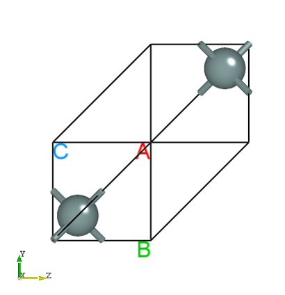
The unit cell information after relaxation can be found in the latestStructure.as file:
1Total number of atoms
22
3Lattice
40.0000000000000000    2.7500000000000000    2.7500000000000000
52.7500000000000000    0.0000000000000000    2.7500000000000000
62.7500000000000000    2.7500000000000000    0.0000000000000000
7Direct
8Si  0.8801735223171917  0.8748246492235915  0.8748246492235915
9Si  0.1298264776828063  0.1251753507764085  0.1251753507764085
This structural relaxation calculation performed 3 ionic steps. In the final relaxed configuration, the x-coordinate of the manually moved Si atom was corrected.
备注
The single-machine DS-PAW execution command is the software name + input file name. If your input file name is abc.in, simply execute DS-PAW abc.in.
The convergence criterion for this relaxation calculation is chosen as atomic force. If energy is to be used as the convergence criterion, you can set relax.convergenceType = energy.
2.2 SCF Self-Consistent Calculation
Self-consistent calculations yield the charge density and wavefunction files for a specific crystal. The charge density file is then used for subsequent calculations of electronic structure properties such as band structure and density of states. It is crucial to note that self-consistent field (SCF) calculations must precede electronic structure calculations such as band structure and density of states calculations. The charge density obtained from the SCF calculation is required for subsequent band structure and density of states calculations.
Input File Preparation for Self-Consistent Calculation of \(Si\) Atom
The input files include the parameter file scf.in and the structure file structure.as. scf.in is shown below:
 1# task type
 2task = scf
 3#system related
 4sys.structure = structure.as
 5sys.symmetry = true
 6sys.functional = PBE
 7sys.spin = none
 8#scf related
 9cal.methods = 2
10cal.smearing = 1
11cal.ksamping = G
12cal.kpoints = [10, 10, 10]
13cal.cutoffFactor = 1.5
14#outputs
15io.charge = true
16io.wave = true
scf.in Input Parameters for Self-Consistent Field Calculation:
task: Sets the calculation type; this calculation is a scf self-consistent field calculation.cal.cutoffFactor: Sets the coefficient forcal.cutoff. The cutoff energy used in the calculation is equal tocal.cutoff*cal.cutoffFactor.io.charge: Controls the output of the charge density file.io.wave: Controls the switch for outputting the wavefunction file;
The structure.as file is referenced as follows:
1Total number of atoms
22
3Lattice
40.00 2.75 2.75
52.75 0.00 2.75
62.75 2.75 0.00
7Direct
8Si -0.125000000 -0.125000000 -0.125000000
9Si 0.125000000 0.125000000 0.125000000
A standard self-consistent calculation usually takes the relaxed structure obtained from structural relaxation as the structural input.
备注
To save ELF and potential data in structure relaxation and self-consistent calculations, simply set io.elf and io.potential to true;
To add a background charge to the system during the calculation, you can directly set the ``sys.electron`` parameter, which specifies the total number of valence electrons.
Run the program.
Once you have prepared the input files scf.in and structure.as, upload them to the server and run the DS-PAW scf.in calculation as described in Structure Relaxation.
Analysis of the calculation results
Based on the above input files, the following output files will be generated after the calculation is completed: DS-PAW.log, scf.h5, rho.bin, wave.bin, and rho.h5.
DS-PAW.log : The log file obtained after the DS-PAW calculation, recording the main information such as energy iteration in the self-consistent calculation;
scf.h5 : The h5 output file for the self-consistent field (SCF) calculation. See Output File Format Specification for a structure analysis.
rho.bin : Binary file of charge density, used for subsequent post-processing calculations;
rho.h5 : The h5 format file of charge density, which can be easily converted to a format readable by VESTA (see Auxiliary Tool User Guide) for visualizing the charge density information.
wave.bin : Binary file of wavefunctions, used for subsequent calculations;
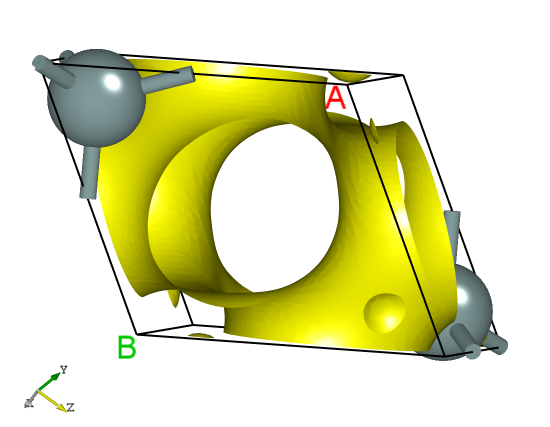
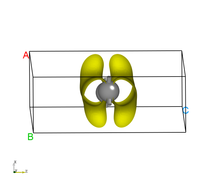
The rho.h5 file can be converted to a format supported by VESTA software via a Python script. See the Auxiliary Tool User Guide section for details. The processing yields 1D, 2D, and 3D charge density plots, with the 3D plot expected to look similar to the following:
2.3 band structure calculation
There are two common ways to perform band calculations: a two-step approach using task=band and a one-step approach using task=scf. This section will use the Si system as an example to illustrate the parameter settings for both methods.
\(Si\) band structure calculation input file
task = band two-step calculation
The input file contains the parameter files scf.in and band.in, the structure file structure.as. The scf.in settings are consistent with the self-consistent calculation in the previous section, and the band.in parameters are as follows:
 1# task type
 2task = band
 3#system related
 4sys.structure = structure.as
 5sys.symmetry = true
 6sys.functional = PBE
 7sys.spin = none
 8
 9cal.iniCharge = ./rho.bin
10cal.methods = 2
11cal.smearing = 1
12cal.cutoffFactor = 1.5
13cal.totalBands = 12
14
15#band related
16band.kpointsLabel= [G,X,W,K,G,L]
17band.kpointsCoord= [0, 0, 0, 0.5, 0, 0.5, 0.5, 0.25, 0.75, 0.375, 0.375, 0.75, 0, 0, 0, 0.5, 0.5, 0.5]
18band.kpointsNumber= [30, 30, 30, 30, 30]
Introduction of input parameters for band.in:
In band calculations, you can generally retain the parameters from sys. and cal. in band.in and then set the specific parameters for the band structure calculation:
task: Specifies the calculation type, which is a band structure calculation in this case.cal.iniCharge: Sets the path to the charge density file, supporting both absolute and relative paths. Here, ./ refers to the rho.bin file in the current directory.
A new set of band-related parameters has been added for band calculations, and these parameters are only effective during band calculations:
band.kpointsLabel: Sets the labels for high-symmetry points during band structure calculation, oneband.kpointsLabelcorresponds to oneband.kpointsCoord;band.kpointsCoord: Set the fractional coordinates of high-symmetry points for band structure calculations, with each group consisting of three numbers;band.kpointsNumber: Sets the number of k-points between every two adjacent high-symmetry points. There are two ways to set this parameter:When the parameter is set as band.kpointsNumber= [30, 30, 30, 30, 30], the number of k-points between all high symmetry points is 30;
When band.kpointsNumber= [30] is set, the number of k-points between high symmetry points G and X is 30, and the k-point density is determined accordingly; uniform k-point sampling is then performed between high symmetry points X and W, W and K, K and G, and G and L. The actual number of k-points can be found in the parameter printing section of DS-PAW.log.
band.EfShift: Determines whether to read the EFermi from rho.bin as the EFermi in the band calculation output. The default is true, which means reading EFermi from rho.bin.
structure.as file is the same as in the self-consistent calculation. (See Section 2.2)
备注
When performing two-step calculations, the parameters cal.cutoffFactor and cal.cutoff in scf.in and band.in must be consistent, otherwise, a mismatch of grid data will occur.
cal.iniCharge specifies the path to the charge density file rho.bin generated by the SCF calculation.
task = scf: one-step calculation
The input file contains the parameter file scf.in and the structure file structure.as. The parameters for scf.in are as follows:
 1# task type
 2task = scf
 3#system related
 4sys.structure = structure.as
 5sys.symmetry = true
 6sys.functional = PBE
 7sys.spin = none
 8#scf related
 9cal.methods = 2
10cal.totalBands = 12
11cal.smearing = 1
12cal.ksamping = G
13cal.kpoints = [10, 10, 10]
14cal.cutoffFactor = 1.5
15#outputs
16io.charge = true
17io.wave = true
18#band related
19io.band=true
20band.kpointsLabel= [G,X,W,K,G,L]
21band.kpointsCoord= [0, 0, 0, 0.5, 0, 0.5, 0.5, 0.25, 0.75, 0.375, 0.375, 0.75, 0, 0, 0, 0.5, 0.5, 0.5]
22band.kpointsNumber= [30, 30, 30, 30, 30]
备注
For one-step band calculations, the result file is scf.h5. The band data is stored in the scf.h5 file, which can be directly processed by the bandplot.py script in Auxiliary Tool User Guide.
io.band=true is only effective when task=scf.
When io.band is enabled, setting cal.iniCharge = ./rho.bin is no longer needed, and the calculation of high-symmetry points in k-space will be performed simultaneously during the scf calculation.
Two types of k-points need to be specified in the scf.in file: cal.kpoints for self-consistent field (SCF) calculations and band.kpoints parameters for band structure calculations. Both sets of k-points are required.
Run the program.
For the two-step calculation example, upload the parameter control files scf.in, band.in, and the structure file structure.as to the server. Then, execute DS-PAW scf.in and DS-PAW band.in sequentially, as described in the structure relaxation section.
Analysis of the calculation results.
Based on the input files mentioned above, the calculation will generate output files such as DS-PAW.log, scf.h5, and band.h5.
DS-PAW.log: The log file obtained after the DS-PAW band structure calculation, which can be directly read to get important information such as band gap, VBM, and CBM.
band.h5 : The h5 output file corresponding to the band calculation; it stores important data such as energy eigenvalues. The specific data structure is detailed in Output File Format Specification.
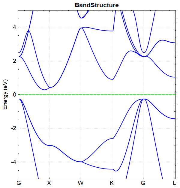
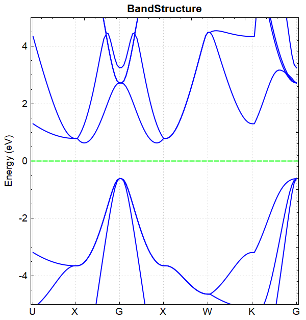
You can use python to process the data in band.h5. For detailed operations, see Auxiliary Tool User Guide. The resulting band structure plot should look like this:
备注
The band diagrams obtained by the one-step and two-step band calculations are consistent.
2.4 pband Projection of Band Calculation
Projected band structures refer to the decomposition of the energy at each k-point of each band into contributions from each atom and its orbitals during a band structure calculation.
Si Projected Band Structure Input File
The input files for the projected band structure calculation include the parameter file pw_band.in, the structure file structure.as, and the binary charge density file rho.bin obtained from the self-consistent calculation. pw_band.in is shown below:
 1# task type
 2task = band
 3#system related
 4sys.structure = structure.as
 5sys.symmetry = true
 6sys.functional = PBE
 7sys.spin = none
 8
 9cal.iniCharge = ./rho.bin
10cal.methods = 2
11cal.smearing = 1
12cal.cutoffFactor = 1.5
13cal.totalBands = 12
14
15#band related
16band.kpointsLabel= [G,X,W,K,G,L]
17band.kpointsCoord= [0, 0, 0, 0.5, 0, 0.5, 0.5, 0.25, 0.75, 0.375, 0.375, 0.75, 0, 0, 0, 0.5, 0.5, 0.5]
18band.kpointsNumber= [30, 30, 30, 30, 30]
19band.project=true
pw_band.in Input Parameters:
The projected band calculation differs from a regular band calculation in that the band.project parameter is set in the calculation parameters:
band.project: Controls whether projection calculations are performed in the band structure calculation;
Run the program
After preparing the input files pw_band.in, structure.as, and rho.bin, upload them to the server for execution. Run DS-PAW pw_band.in following the procedure described in the structural relaxation section.
Analysis Results
Based on the input files mentioned above, after the calculation is completed, output files such as DS-PAW.log and band.h5 will be generated.
DS-PAW.log: The log file generated after the DS-PAW band calculation;
band.h5 : The h5 output file corresponding to the band structure calculation. Projected band data will also be saved in band.h5. See Output File Format Specification for details on the data structure;
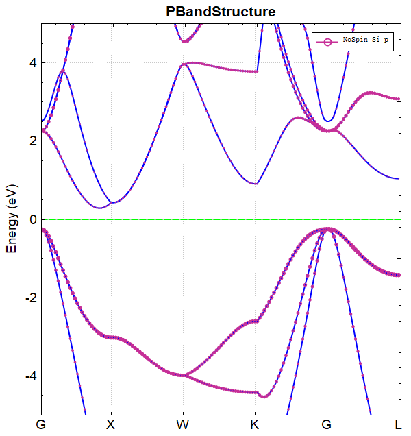
Data processing of band.h5 can be done using python, see Auxiliary Tool User Guide for details. The resulting band structure plot should look like this:
2.5 DOS calculation
Density of states (DOS) calculations can be performed in two ways: a two-step method with task=dos and a one-step method with task=scf. This section uses Si as an example to illustrate the parameter settings for both methods.
Input file for Density of States (DOS) calculation of a Si system
task = dos two-step calculation
The input files include the parameter files scf.in and dos.in, and the structure file structure.as. scf.in is set consistently with the self-consistent calculation, and the parameters in dos.in are as follows:
 1# task type
 2task = dos
 3#system related
 4sys.structure = structure.as
 5sys.symmetry = true
 6sys.functional = PBE
 7sys.spin = none
 8
 9cal.iniCharge = ./rho.bin
10cal.methods = 2
11cal.smearing = 4
12cal.ksamping = G
13cal.kpoints = [20, 20, 20]
14cal.cutoffFactor = 1.5
15
16#dos related
17dos.range=[-10, 10]
18dos.resolution=0.05
dos.in Input Parameters Introduction:
In the DOS calculation, parameters in sys. and cal. can be retained as much as possible in dos.in, then set the specific parameters for DOS calculation:
task: Sets the calculation type. For this calculation, it’s DOS (density of states) calculation.cal.iniCharge: Sets the reading path for the charge density, supporting both absolute and relative paths; here, ./ refers to the rho.bin file in the current directory;cal.kpoints: Sets the k-point grid density. For DOS calculations, it is recommended to increase the k-points to about twice the density used in the self-consistent calculation.
A new set of parameters related to the density of states has been added for DOS calculations, and these parameters are only effective in the DOS calculation:
dos.range: Sets the energy range for the density of states calculation.dos.resolution: Sets the energy interval precision for the density of states calculation. The number of points for the DOS calculation is the difference between dos.range divided by dos.resolution plus 1.
structure.as file is the same as the self-consistent calculation. (See Section 2.2)
备注
When performing a two-step calculation, the parameters `cal.cutoffFactor` and `cal.cutoff` in `scf.in` and `dos.in` must be consistent; otherwise, grid data mismatch issues will occur.
task = scf one-step calculation
The input file includes the parameter file scf.in, the structure file structure.as, and the parameters for scf.in are as follows:
 1# task type
 2task = scf
 3#system related
 4sys.structure = structure.as
 5sys.symmetry = true
 6sys.functional = PBE
 7sys.spin = none
 8#scf related
 9cal.methods = 2
10cal.smearing = 4
11cal.ksamping = G
12cal.kpoints = [10, 10, 10]
13cal.cutoffFactor = 1.5
14#outputs
15io.charge = true
16io.wave = true
17#dos related
18io.dos=true
19dos.range=[-10, 10]
20dos.resolution=0.05
备注
For the one-step DOS calculation, the result file is scf.h5. The DOS data is stored in the scf.h5 file, and you can directly use the Auxiliary Tool User Guide’s dosplot.py script to process the scf.h5 file.
io.dos=true is only effective when task=scf.
When io.dos is enabled, it’s no longer necessary to set cal.iniCharge = ./rho.bin; the DOS is obtained through the self-consistent calculation in this case.
run the program
For the two-step calculation as an example, upload the parameter control files scf.in, dos.in, and the structure file structure.as to the server, and then sequentially run DS-PAW scf.in and DS-PAW dos.in as described in the structure relaxation section.
Analysis of the calculation results
Based on the input files mentioned above, the calculation will generate output files such as DS-PAW.log, scf.h5, and dos.h5.
DS-PAW.log : Log file generated after DS-PAW density of states calculation;
dos.h5 : The h5 file containing the density of states data. For details on its structure, see the Output File Format Specification section.
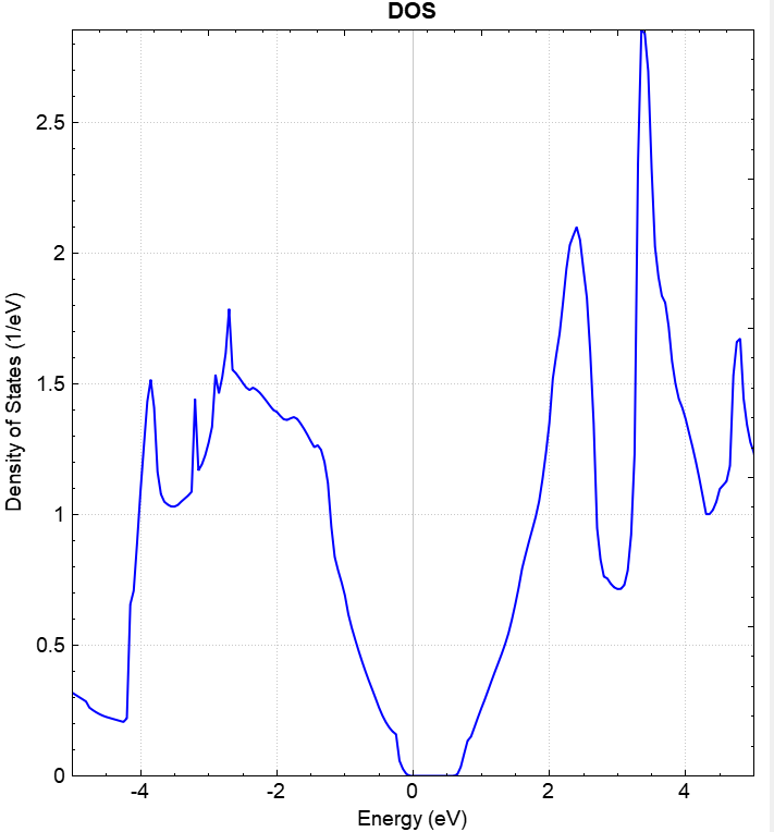
You can process dos.h5 data using python. See the Auxiliary Tool User Guide section for details. The resulting density of states plot should look like this:
2.6 pdos Projected Density of States Calculation
The calculation of projected density of states refers to the process of expanding the density of states at each energy level during the density of states calculation into contributions from each atom and its orbitals.
\(Si\) projected density of states calculation input file
The input files for projected density of states calculations include the parameter file pdos.in, the structure file structure.as, and the charge density file from the self-consistent calculation rho.bin. The pdos.in file is as follows:
 1# task type
 2task = dos
 3#system related
 4sys.structure = structure.as
 5sys.symmetry = true
 6sys.functional = PBE
 7sys.spin = none
 8
 9cal.iniCharge = ./rho.bin
10cal.methods = 2
11cal.smearing = 4
12cal.ksamping = G
13cal.kpoints = [20, 20, 20]
14cal.cutoffFactor = 1.5
15
16#dos related
17dos.range=[-10, 10]
18dos.resolution=0.05
19dos.project = true
Introduction to the input parameters for pdos.in:
The difference between projected density of states and regular density of states lies in the setting of the dos.project parameter within the calculation parameters:
dos.project: Controls the switch for projected calculations in the density of states calculation.
Run the program
After preparing the input files pdos.in, structure.as, and rho.bin, upload the files to the server and run DS-PAW pdos.in as described in the structure relaxation method.
Analysis of the calculation results.
Based on the above input files, the calculation will generate output files such as DS-PAW.log and dos.h5.
DS-PAW.log : The log file generated after the DS-PAW density of states calculation;
dos.h5 : The h5 output file corresponding to the density of states calculation; the projected density of states data is stored in the dos.h5 file. For the specific data structure, see the Output File Format Specification section;
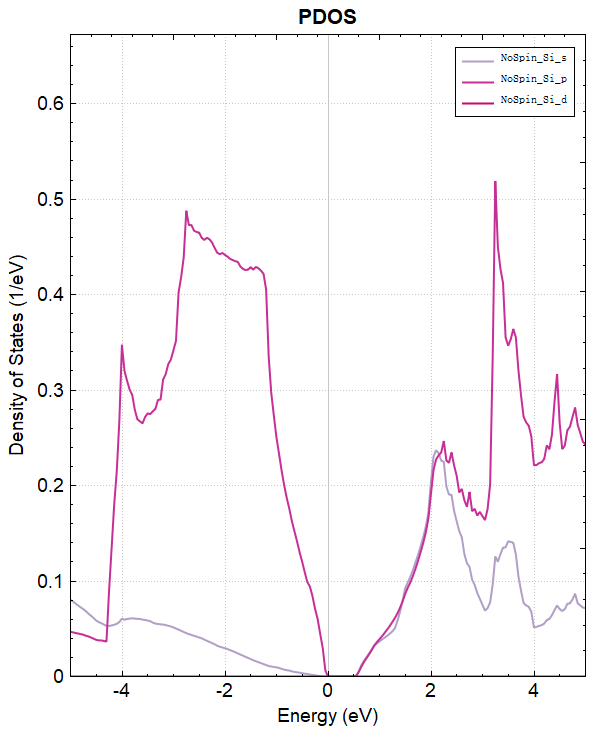
You can process dos.h5 data using python. See Auxiliary Tool User Guide for specific operations. The resulting projected density of states plot should look like the following:
2.7 potential calculation
There are two methods for calculating the potential function: a two-step method using task=potential and a one-step method using task=scf. This section takes the Si system as an example to introduce the corresponding parameter settings for both methods.
Input file for \(Si\) potential function calculation
task = potential two-step calculation
The input files include the parameter file scf.in, potential.in, and the structure file structure.as. scf.in is set up consistently with the self-consistent calculation, while potential.in is configured as follows:
 1# task type
 2task = potential
 3#system related
 4sys.structure = structure.as
 5sys.symmetry = true
 6sys.functional = PBE
 7sys.spin = none
 8
 9cal.iniCharge = ./rho.bin
10cal.methods = 2
11cal.smearing = 1
12cal.ksamping = G
13cal.kpoints = [10, 10, 10]
14cal.cutoffFactor = 1.5
15
16#potential related
17potential.type=all
Introduction of the input parameters in potential.in:
In the potential calculation, you can retain as many parameters as possible from sys. and cal. in potential.in, and then set the specific parameters for the potential calculation:
task: Set the calculation type. This calculation is apotentialpotential function calculation.cal.iniCharge: Sets the path to read the charge density file, supporting both absolute and relative paths. Here, ./ refers to the rho.bin file in the current directory;
New parameters in potential calculation:
potential.type: Controls the type of potential saved. When all is selected, both the electrostatic potential (sum of ionic and Hartree potentials) and the local potential (sum of electrostatic and exchange-correlation potentials) will be saved after the potential calculation is completed.
structure.as file as the self-consistent calculation result. (See Section 2.2)
备注
When performing two-step calculations, the parameters `cal.cutoffFactor` and `cal.cutoff` in both `scf.in` and `potential.in` must be consistent; otherwise, a mismatch in the grid data will occur.
If the system being calculated requires dipole correction, the user needs to add the parameters `corr.dipol = true` and `corr.dipolDirection` in both the self-consistent field (SCF) and potential calculation input files. `corr.dipol = true` enables the dipole correction switch, and `corr.dipolDirection` sets the dipole correction direction; a, b, and c represent the directions along the lattice vectors a, b, and c, respectively.
For a specific example of dipole correction, see the application case: Calculation of Work Function for Au-Al System.
task = scf one-step calculation
The input file contains the parameter file scf.in, the structure file structure.as, and the parameters for scf.in are as follows:
 1# task type
 2task = scf
 3#system related
 4sys.structure = structure.as
 5sys.symmetry = true
 6sys.functional = PBE
 7sys.spin = none
 8#scf related
 9cal.methods = 2
10cal.smearing = 1
11cal.ksamping = G
12cal.kpoints = [10, 10, 10]
13cal.cutoffFactor = 1.5
14#outputs
15io.charge = true
16io.wave = true
17#potential related
18io.potential = true
备注
For the one-step potential calculation, the corresponding result file is scf.h5. In this case, the potential data is stored in the scf.h5 file, and you can directly call the potential processing script of Auxiliary Tool User Guide to analyze the scf.h5 file.
io.potential=true is only effective when task=scf.
Run the program.
For the two-step calculation as an example, upload the parameter control file scf.in, potential.in, and structure file structure.as to the server, and then execute DS-PAW scf.in and DS-PAW potential.in sequentially according to the method described in structure relaxation.
Analysis of the calculation results
Based on the input files mentioned above, the calculation will generate the following output files: DS-PAW.log, scf.h5, and potential.h5.
DS-PAW.log : Log file generated after DS-PAW potential calculation.
potential.h5 : The h5 output file corresponding to the potential calculation, with specific structure detailed in Output File Format Specification.
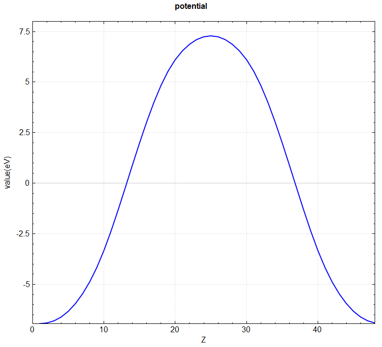
You can use a Python script to convert the potential.h5 format to a format supported by VESTA software, or directly use the script to perform in-plane averaging of the 3D potential function. For specific operations, see the Auxiliary Tool User Guide section. The processed vacuum direction potential curve is shown below:
2.8 elf calculation of electronic local density
There are two ways to calculate the electron localization function (ELF): a two-step approach with task=elf and a one-step approach with task=scf. This section uses a Si system as an example to illustrate the corresponding parameter settings for both methods.
\(Si\) Electronic Localized Function calculation input file
task = elf two-step calculation
Input files include parameter files scf.in and ELF.in, and structure file structure.as. scf.in settings are consistent with self-consistent calculations, while ELF.in settings are as follows:
 1# task type
 2task = elf
 3#system related
 4sys.structure = structure.as
 5sys.symmetry = true
 6sys.functional = PBE
 7sys.spin = none
 8
 9cal.iniCharge = ./rho.bin
10cal.methods = 2
11
12cal.smearing = 1
13cal.ksamping = G
14cal.kpoints = [10, 10, 10]
15cal.cutoffFactor = 1.5
ELF.in Input Parameter Description:
In ELF calculations, it is recommended to retain the sys. and cal. parameters in ELF.in as much as possible:
task: Sets the calculation type; this calculation is an ELF calculation.cal.iniCharge: Sets the reading path of the charge density file. Both absolute and relative paths are supported. Here, “./” represents the rho.bin file in the current path;
The structure.as file is the same as that used in the self-consistent calculation (see Section 2.2).
备注
For two-step calculations, the parameters `cal.cutoffFactor` and `cal.cutoff` in both `scf.in` and `ELF.in` must be consistent; otherwise, grid data mismatch will occur.
ELF calculation does not support non-collinear calculations.
task = scf one-step calculation
The input files include the parameter file scf.in, the structure file structure.as. The scf.in parameters are as follows:
 1# task type
 2task = scf
 3#system related
 4sys.structure = structure.as
 5sys.symmetry = true
 6sys.functional = PBE
 7sys.spin = none
 8#scf related
 9cal.methods = 2
10cal.smearing = 1
11cal.ksamping = G
12cal.kpoints = [10, 10, 10]
13cal.cutoffFactor = 1.5
14#outputs
15io.charge = true
16io.wave = true
17#elf related
18io.elf = true
备注
The output file for a single-step calculation of electron localization density is scf.h5. The electron localization density data is stored in this file and can be directly analyzed using the electron localization density processing scripts in Auxiliary Tool User Guide.
io.elf=true only takes effect when task=scf.
ELF calculation does not support non-collinear calculations.
Run the program
For a two-step calculation example, upload the parameter control files scf.in, ELF.in, and the structure file structure.as to the server. Then, execute DS-PAW scf.in and DS-PAW ELF.in sequentially, as described in the structural relaxation section.
Analysis Results
Based on the input files above, after the calculation is completed, output files such as DS-PAW.log, scf.h5, and elf.h5 will be generated.
DS-PAW.log : Log file generated after the DS-PAW local density calculation.
elf.h5 : ELF calculation output file in h5 format; details of the structure are described in Output File Format Specification.
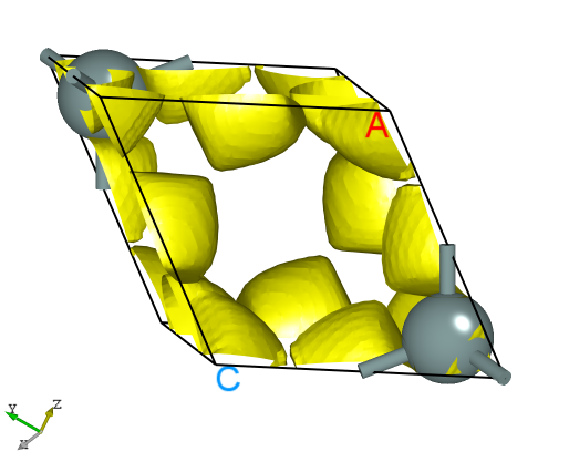
The elf.h5 format can be converted to a format supported by the VESTA software using a python script; see the Auxiliary Tool User Guide section for details. The resulting 3D electron localization density map should look like this:
2.9 pcharge Part Charge Density Calculation
This section will analyze the charge density of specific bands at specified k-points, using graphene as an example. It details the preparation of partial charge density calculations after self-consistent field calculations, and the subsequent analysis through plotting.
Input file for partial charge density calculation of graphene
The input files include the parameter file pcharge.in and the structure file structure.as, the charge density file rho.bin and the wavefunction file wave.bin obtained from self-consistent calculations, and pcharge.in is as follows:
 1# task type
 2task = pcharge
 3#system related
 4sys.structure = structure.as
 5sys.symmetry = true
 6sys.functional = PBE
 7sys.spin = none
 8
 9cal.methods = 2
10cal.smearing = 1
11cal.ksamping = G
12cal.kpoints = [9, 9, 1]
13cal.cutoffFactor = 1.5
14cal.iniCharge = ./rho.bin
15cal.iniWave = ./wave.bin
16
17#pcharge related
18pcharge.bandIndex = [4,5]
19pcharge.kpointsIndex = [12]
20pcharge.sumK= false
pcharge.in input parameters introduction:
In the partial charge density calculation, parameters from sys. and cal. can be retained in pcharge.in as much as possible, and then the specific parameters for partial charge density calculation can be set:
task: Sets the calculation type, which is partial charge density calculation in this case;cal.iniCharge: Sets the path for reading the charge density file, supporting absolute and relative paths. Here, ./ refers to the rho.bin file in the current directory.cal.iniWave: Sets the reading path for the wave function file, supporting both absolute and relative paths. Here, ./ indicates the wave.bin file under the current path;pcharge.bandIndex: Specifies the band indices for charge density analysis. Here, [4,5] indicates that the charge density of band 4 and band 5 will be analyzed.pcharge.kpointsIndex: Sets the K-point index for charge density analysis. Here, [12] indicates that the K-point index is 12 when analyzing the charge density of two bands.pcharge.sumK: Controls whether to sum the band data of all analyzed K-points. Here, false means no summation.
structure.as file is referenced as follows:
1Total number of atoms
22
3Lattice
42.46120000 0.00000000 0.00000000
5-1.23060000 2.13146172 0.00000000
60.00000000 0.00000000 6.70900000
7Cartesian
8C  0.61530000  0.35524362  3.35450000
9C  0.61530000  1.77621810  3.35450000
备注
Partial charge density calculation is performed in two steps, with the second step requiring reading the charge density file rho.bin and the wavefunction file wave.bin from the self-consistent calculation.
run program execution
Prepare the input files pcharge.in, structure.as, and the self-consistent calculation results rho.bin and wave.bin, upload them to the server for execution, and run DS-PAW pcharge.in following the method described in structure relaxation.
Analysis of the calculation results
Based on the input files described above, the calculation will generate output files such as DS-PAW.log and pcharge.h5.
DS-PAW.log : The log file generated after the DS-PAW partial charge density calculation.
pcharge.h5 : The HDF5 data file after the partial charge density calculation is completed. The charge density data for two bands is saved in pcharge.h5 at this time. The specific data structure can be found in the Output File Format Specification section.
You can process the data in pcharge.h5 using python. See Auxiliary Tool User Guide for specific operations. The charge density plot for band 4 at k-point index 12 should look like this:
2.10 hse hybrid functional calculation
This section will demonstrate the calculation of hybrid functional band structures using the direct band structure calculation method within the DS-PAW code, using the Si system as an example. We will observe the changes in the band gap after performing hybrid functional calculations.
\(Si\) Hybrid Functional Calculation Input File
The input file includes the parameter file ioband.in and the structure file structure.as. The content of ioband.in is as follows:
 1# task type
 2task = scf
 3#system related
 4sys.structure = structure.as
 5sys.symmetry = true
 6sys.spin = none
 7#scf related
 8cal.methods = 1
 9cal.totalBands = 12
10cal.smearing = 1
11cal.ksamping = G
12cal.kpoints = [5, 5, 5]
13cal.cutoffFactor = 1.5
14#band related
15io.band = true
16band.kpointsCoord=[0.62500000,0.25000000,0.62500000,0.50000000,0.00000000,0.50000000,0.00000000,0.00000000,0.00000000,0.50000000,0.00000000,0.50000000,0.50000000,0.25000000,0.75000000,0.37500000,0.37500000,0.75000000,0.00000000,0.00000000,0.00000000]
17band.kpointsLabel = [U,X,G,X,W,K,G]
18band.kpointsNumber = [20,20,20,20,20,20]
19band.project = false
20#HSE related
21sys.hybrid=true
22sys.hybridType=HSE06
23#outputs
24io.charge = true
25io.wave = true
ioband.in Input Parameters:
In hybrid functional calculations, you can generally preserve the sys. and cal. parameters in ioband.in as much as possible, and then set the specific parameters for hybrid functional calculations:
sys.hybrid: Controls the switch for hybrid functional calculations. true indicates the introduction of hybrid functional calculations;sys.hybridType: Sets the type of hybrid functional, which is HSE06 in this case;
structure.as file is the same as in the self-consistent calculation. (See Section 2.2)
备注
Unlike regular calculations where the functional type is set using `sys.functional`, hybrid functional calculations control the hybrid functional type via the `sys.hybridType` parameter.
Hybrid functional calculations only support tasks ‘scf’ and ‘relax’. Therefore, band structure calculations with hybrid functionals can only be performed in a single-shot manner.
It is recommended to use damped MD/conjugated gradient methods for electronic self-consistent field (SCF) calculations with hybrid functionals, corresponding to setting the parameter cal.methods = 4/5.
Hybrid functional calculations can also use the block Davidson method for electronic self-consistent calculations, i.e., cal.methods = 1 in this example. In this case, the scf.mixType parameter will default to Kerker.
Run the program.
Prepare the input files ioband.in and structure.as and upload them to the server to run. Execute DS-PAW ioband.in as described in Structure Relaxation.
Analysis of calculation results
After the calculation is completed based on the input files mentioned above, output files such as DS-PAW.log and scf.h5 will be generated. The method for processing scf.h5 is the same as the band structure calculation method (see Section 2.3), and the resulting band structure plot should look like the following:
Modifying the hybrid functional Alpha coefficient
The hybrid functional method shown in Section 2.10.1 is HSE06, with a corresponding hybrid functional coefficient of sys.hybridAlpha = 0.25. Adjust the sys.hybridAlpha parameter and perform the following two calculations:
Modify the parameter in scf.in and band.in:
sys.hybridAlpha = 0.20Modify the parameter in scf.in and band.in:
sys.hybridAlpha = 0.30
Obtain the following band structure comparison:
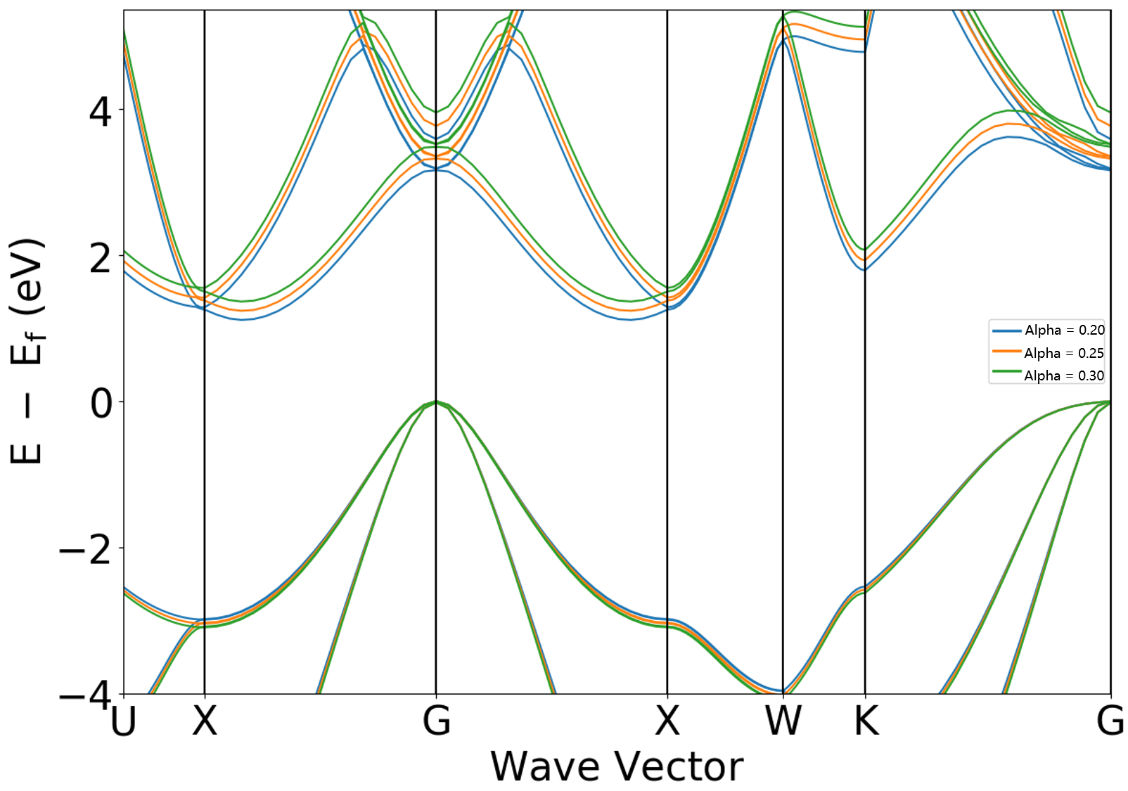
Analysis of the figure shows that increasing the sys.hybridAlpha coefficient leads to a further increase in the band gap.
The band gap values of 1.1146, 1.2394, and 1.3665 eV can be read from the DS-PAW.log file when sys.hybridAlpha is set to 0.20, 0.25, and 0.30, respectively.
2.11 van der Waals Correction Calculation
This section will use the structural relaxation of a graphite system as an example to illustrate how to correctly set up van der Waals corrections in DS-PAW, and will compare and analyze the results with and without the van der Waals correction.
Graphite structure relaxation input file
When relaxing graphite, you can choose to correct van der Waals forces using a semi-empirical method or a functional correction method. The parameter settings for both methods are described below.
Empirical Correction
The input files include the parameter file relax.in and the structure file structure.as. relax.in is shown below:
 1# task type
 2task = relax
 3#system related
 4sys.structure = structure.as
 5sys.symmetry = true
 6sys.functional = PBE
 7sys.spin = none
 8#scf related
 9cal.methods = 1
10cal.smearing = 1
11cal.ksamping = G
12cal.kpoints = [21, 21, 7]
13cal.cutoff  = 600
14scf.convergence = 1.0e-05
15#relax related
16relax.max =  60
17relax.freedom = all
18relax.convergence =  0.01
19relax.methods = CG
20#vdw related
21corr.VDW = true
22corr.VDWType = D3G
relax.in Input Parameters:
In the van der Waals correction calculation, try to keep the parameters of sys. and cal. in relax.in, then set the parameters specific to the van der Waals correction calculation.
corr.VDW: Controls the switch for the semi-empirical van der Waals correction, true indicates it is turned on;corr.VDWType: Sets the type of van der Waals correction, D3G representing the DFT-D3 method of Grimme;
The structure.as file is referenced as follows:
 1Total number of atoms
 24
 3Lattice
 42.46729136 0.00000000 0.00000000
 5-1.23364568 2.13673699 0.00000000
 60.00000000 0.00000000 7.80307245
 7Cartesian
 8C 0.00000000 0.00000000 1.95076811
 9C 0.00000000 0.00000000 5.85230434
10C 0.00000000 1.42449201 1.95076811
11C 1.23364689 0.71224492 5.85230434
备注
When correcting van der Waals forces using semi-empirical methods, different types of exchange-correlation functionals can be selected. The selectable values for sys.functional are PBE/REVPBE/RPBE/PBESOL.
DS-PAW supports using semi-empirical methods to correct van der Waals forces while simultaneously enabling hybrid functional calculations.
Functional Correction
The input file corresponding to the functional correction, relax.in, can be structured as follows:
 1# task type
 2task = relax
 3#system related
 4sys.structure = structure.as
 5sys.symmetry = true
 6sys.spin = none
 7#scf related
 8cal.methods = 1
 9cal.smearing = 1
10cal.ksamping = G
11cal.kpoints = [21, 21, 7]
12cal.cutoff  = 600
13scf.convergence = 1.0e-05
14#relax related
15relax.max =  60
16relax.freedom = all
17relax.convergence =  0.01
18relax.methods = CG
19#vdw related
20sys.functional = vdw-optPBE
relax.in Input Parameter Introduction:
In calculations with van der Waals corrections, parameters related to sys. and cal. can generally be kept in the relax.in file. Subsequently, set the specific parameters for the van der Waals correction calculation.
sys.functional: Controls the type of functional. When selecting a functional that includes van der Waals correction, simply set the vdw-series functional parameters. This example uses the vdw-optPBE functional. Supported functional types are listed in the Parameters Explanation section.
备注
From a theoretical perspective, there are two different ways to correct for van der Waals interactions, corresponding to the parameters corr.VDW = true (semi-empirical correction) and sys.functional = vdw-… (functional correction), respectively.
run the program
For the example of a semi-empirical correction, after preparing the input file, upload the relax.in and structure.as files to the server and run the DS-PAW relax.in file as described in structure relaxation.
Analysis of calculation results
After the calculation based on the above input file, output files such as DS-PAW.log, relax.h5, and latestStructure.as will be generated. (Another set of calculations without considering van der Waals corrections is added for comparison.)
Drag latestStructure.as into Device Studio to view the structure. The lattice constants after relaxation are shown in the following table. By comparison, it is found that the value of the lattice vector c obtained from structural relaxation with the addition of van der Waals correction is closer to the experimental results reported in :footcite:p:Rgo2015ComparativeSO.
Procedure
a (Å)
c (Å)
vdw-D3G this work
2.463
6.954
PBE this work
2.464
7.914
Experiment
2.462
6.707
2.12 Optical Property Calculations
There are two ways to perform optical calculations: a two-step approach with task=optical and a one-step approach with task=scf. This section will use the Si system as an example to illustrate how to calculate optical properties in DS-PAW and analyze a series of optical properties by plotting them.
\(Si\) optical property calculation input file
task = optical two-step calculation
The input files contain the parameter file scf.in, optical.in, and the structure file structure.as. The settings in scf.in are consistent with the self-consistent calculation, and the settings in optical.in are as follows:
optical.in is set as follows:
 1# task type
 2task = optical
 3#system related
 4sys.structure = structure.as
 5sys.symmetry = true
 6sys.functional = PBE
 7sys.spin = none
 8#scf related
 9cal.methods = 1
10cal.smearing = 1
11cal.ksamping = G
12cal.kpoints = [12, 12, 12]
13cal.cutoffFactor = 1.5
14cal.iniCharge = ./rho.bin
15
16#optical related
17optical.grid = 2000
18optical.sigma = 0.05
19optical.smearing = 1
In optical calculations, you can retain the parameters of sys. and cal. as much as possible in :guilabel:`optical.in and then set the parameters specific to optical calculations:
task: Sets the calculation type, this calculation istask = optical: optical calculation;cal.iniCharge: Sets the path to read the charge density file, supporting both absolute and relative paths. Here, ./ indicates the rho.bin file in the current directory;optical.grid: Specifies the number of grid points within the energy range for DS-PAW optical property calculations, in this case, 2000.optical.sigma: Determines the broadening width when using the broadening algorithm specified byoptical.smearing, which is 0.05 in this example.optical.smearing: Specifies the smearing algorithm used for energy broadening in optical calculations, which is 1 in this case.
task = scf one-step calculation
The input file contains the parameter file scf.in and the structure file structure.as. The settings for scf.in are as follows:
 1# task type
 2task = scf
 3#system related
 4sys.structure = structure.as
 5sys.symmetry = true
 6sys.functional = PBE
 7sys.spin = none
 8#scf related
 9cal.methods = 1
10cal.smearing = 1
11cal.ksamping = G
12cal.kpoints = [12, 12, 12]
13cal.cutoffFactor = 1.5
14#optical related
15io.optical = true
scf.in Input parameters introduction:
In optical property calculations, you can retain as many sys. and cal. parameters as possible in scf.in, and then set the specific parameters for optical property calculations:
io.optical: Controls the switch for optical property calculations. When io.optical=true, the system performs calculations for optical properties;
structure.as file as in self-consistent calculation. (See Section 2.2)
run the program
For the two-step calculation as an example, after preparing the input files, upload the scf.in, optical.in, and structure.as files to the server and run them. Execute DS-PAW scf.in and optical.in as described in the structure relaxation.
Analysis of calculation results
Based on the input files mentioned above, the calculation will generate output files including DS-PAW.log, scf.h5, and optical.h5.
DS-PAW.log : Log file generated after DS-PAW optical properties calculation.
optical.h5 : The h5 data file after the optical properties calculation is completed. Note that the name of the h5 file is strictly consistent with the task type. For the data structure of the h5 file, please refer to Output File Format Specification.
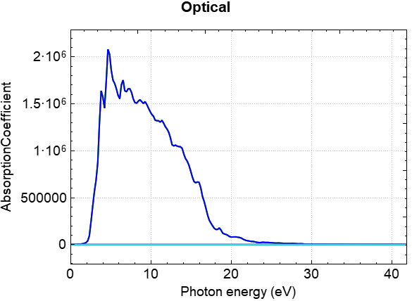
You can use python to process the data from optical.h5 or the one-step calculation result scf.h5. For specific operations, refer to the Auxiliary Tool User Guide section. Processing allows you to obtain curves of the real part of the dielectric function, the imaginary part of the dielectric function, the absorption coefficient, the extinction coefficient, the conductivity, the reflectivity, the refractive index, and the energy loss as a function of energy. Taking the absorption coefficient curve as an example, the resulting curve should look like the following:
2.13 Frequency Calculation
This section will use the \(CO\) molecule as an example to illustrate how to perform frequency calculations in DS-PAW.
\(CO\) frequency calculation input file
The input file contains the parameter file frequency.in and the structure file structure.as, with frequency.in as follows:
 1# task type
 2task = frequency
 3#system related
 4sys.structure = structure.as
 5sys.symmetry = true
 6sys.functional = PBE
 7sys.spin = none
 8#scf related
 9cal.methods = 2
10cal.smearing = 1
11cal.ksamping = MP
12cal.kpoints = [9, 9, 9]
13cal.cutoffFactor = 1.5
14scf.convergence = 1.0e-6
15#frequency related
16frequency.dispOrder = 1
17frequency.dispRange = 0.02
18#outputs
19io.charge = false
20io.wave = false
Introduction to input parameters for frequency.in:
In the frequency calculation, you can retain as many parameters from sys. and cal. as possible in frequency.in, and then set the parameters specific to the frequency calculation:
task: Set the calculation type, which is frequency calculation for this run;frequency.dispOrder: Sets the atomic vibration mode for frequency calculations. 1 corresponds to the central difference method, i.e., 2 atomic vibration modes: the displacement of atoms in each Cartesian direction is±frequency.dispRange; 2 corresponds to 4 atomic vibration modes: the displacement of atoms in each Cartesian direction is±frequency.dispRangeand±2*frequency.dispRange;frequency.dispRange: Sets the displacement magnitude of atoms during frequency calculation.
The structure.as file is referenced as follows:
1Total number of atoms
22
3Lattice
48.0 0.0 0.0
50.0 8.0 0.0
60.0 0.0 8.0
7Cartesian  Fix_x Fix_y Fix_z
8O 0 0 0       T T F
9C 0 0 1.143   T T F
备注
Increase the convergence accuracy of the self-consistent field (SCF) calculation during frequency calculation. It is recommended to set it to 1.0e-6 or higher.
Since C and O atoms are fixed in the x and y directions, they can only move in the z direction.
run program execution
After preparing the input files, upload the :guilabel:`frequency.in and :guilabel:`structure.as files to the server and run :guilabel:`DS-PAW frequency.in as described in Structure Relaxation.
Analysis of calculation results
Based on the input files mentioned above, the calculation will generate output files including DS-PAW.log, frequency.h5, and frequency.txt.
DS-PAW.log : The log file generated after the DS-PAW frequency calculation.
frequency.h5 : The h5 data file after frequency calculation. The frequency data is stored in this file at this time. For the specific data structure, see the Output File Format Specification section.
frequency.txt: The txt text file generated after frequency calculation, which writes frequency-related data. This file contains the same data as frequency.h5, making it easy for users to quickly access the information.
The following data can be obtained from frequency.txt:
Frequency |
THz |
2PiTHz |
cm-1 |
meV |
1 f |
63.844168 |
401.144726 |
2129.612084 |
264.038342 |
2 f/i |
0.051335 |
0.322546 |
1.712346 |
0.212304 |
CO moves only along the z-axis for two atoms, resulting in only two frequencies. Based on the table above, one vibrational mode has a frequency of approximately 63.8 THz, and the other is a near-zero imaginary frequency. Generally, imaginary frequencies less than 2 THz can be considered negligible.
2.14 Calculating elastic constants
This section will use the Si system as an example to demonstrate how to perform elastic calculations in DS-PAW.
\(Si\) Input file for elastic constant calculation
The input file includes the parameter file elastic.in and the structure file structure.as, with elastic.in as follows:
 1# task type
 2task = elastic
 3#system related
 4sys.structure = structure.as
 5sys.symmetry = true
 6sys.functional = PBE
 7sys.spin = none
 8#scf related
 9cal.methods = 1
10cal.smearing = 1
11cal.ksamping = G
12cal.kpoints = [5, 5, 5]
13cal.cutoffFactor = 1.5
14scf.convergence = 1.0e-6
15#frequency related
16elastic.dispOrder = 1
17elastic.dispRange = 0.01
18#outputs
19io.charge = false
20io.wave = false
elastic.in Input Parameter Introduction:
In elastic calculations, you can generally preserve the sys. and cal. parameters in elastic.in as much as possible, and then set the parameters specific to the elastic calculation:
task: Set the calculation type; this calculation is an elastic calculation.elastic.dispOrder: Set the method of atomic vibration for elastic calculations; 1 corresponds to the central difference method;elastic.dispRange: Set the magnitude of atomic displacement for elastic calculations;
structure.as The file is referenced as follows:
 1Total number of atoms
 28
 3Lattice
 45.43070000 0.00000000 0.00000000
 50.00000000 5.43070000 0.00000000
 60.00000000 0.00000000 5.43070000
 7Cartesian
 8Si 0.67883750 0.67883750 0.67883750
 9Si 3.39418750 3.39418750 0.67883750
10Si 3.39418750 0.67883750 3.39418750
11Si 0.67883750 3.39418750 3.39418750
12Si 2.03651250 2.03651250 2.03651250
13Si 4.75186250 4.75186250 2.03651250
14Si 4.75186250 2.03651250 4.75186250
15Si 2.03651250 4.75186250 4.75186250
备注
When performing elastic calculations, the convergence accuracy of self-consistent calculations should be increased. It is recommended to set it to 1.0e-6 or higher.
Fixed atoms are not supported in elastic calculations.
run program execution
After preparing the input files, upload the :guilabel:`elastic.in and :guilabel:`structure.as files to the server and run :guilabel:`DS-PAW elastic.in following the method described in Structure Relaxation.
Analysis of the calculation results.
After the calculation based on the input files mentioned above, the following three files will be generated: DS-PAW.log, elastic.h5, and elastic.txt.
DS-PAW.log: Log file generated after the DS-PAW elastic calculation;
elastic.h5 : h5 data file generated after the elasticity calculation. The elastic modulus is stored in elastic.h5. For detailed data structure, please refer to Output File Format Specification;
elastic.txt : A txt text file generated after the elasticity calculation. This file contains elasticity-related data, consistent with the elastic.h5 file, for easy user access.
The elastic constant matrix obtained from the elastic.txt file is as follows:
Stiffness Elasticity Matrix:
158.7644
62.9858
62.9858
0.0000
-0.0000
0.0000
62.9858
158.7644
62.9858
0.0000
0.0000
0.0000
62.9858
62.9858
158.7644
-0.0000
0.0000
0.0000
0.0000
0.0000
-0.0000
75.8807
-0.0000
0.0000
-0.0000
0.0000
0.0000
-0.0000
75.8807
-0.0000
0.0000
0.0000
0.0000
0.0000
-0.0000
75.8807
Flexibility Elasticity Matrix:
0.0081
-0.0023
-0.0023
-0.0000
0.0000
-0.0000
-0.0023
0.0081
-0.0023
-0.0000
-0.0000
0.0000
-0.0023
-0.0023
0.0081
0.0000
-0.0000
0.0000
-0.0000
-0.0000
0.0000
0.0132
0.0000
-0.0000
0.0000
-0.0000
-0.0000
0.0000
0.0132
0.0000
-0.0000
0.0000
0.0000
-0.0000
0.0000
0.0132
Bulk Modulus, Shear Modulus, Young’s Modulus, and Poisson’s Ratio:
Properties
Vogit
Reuss
Hill
BulkModulus(GPa)
94.9120
94.9120
94.9120
ShearModulus(GPa)
64.6841
61.5016
63.0929
YoungModulus(GPa)
158.1297
151.7315
154.9452
PoissonRatio
0.2223
0.2336
0.2279
The Si system is cubic. This crystal system has three independent matrix elements: C11, C12, and C44, corresponding to 158.7644, 62.9858, and 75.8807 in the table, respectively.
2.15 NEB Transition State Calculation
This section introduces how to perform transition state calculations (CI-NEB) in DS-PAW using the example of H diffusion on the Pt(100) surface, and how to analyze the results graphically.
Transition state calculation input file \(Pt\)
The input files include a parameter file, neb.in, and multiple structure files, structureNo.as. The neb.in file is as follows:
 1task = neb
 2
 3sys.structure = structure.as
 4sys.functional  = PBE
 5sys.spin = none
 6sys.symmetry = true
 7
 8cal.ksamping = G
 9cal.kpoints = [3,3,1]
10cal.cutoffFactor = 1.0
11cal.smearing = 1
12cal.sigma = 0.05
13
14neb.freedom = atom
15neb.springK = 5
16neb.images = 3
17neb.iniFin = true
18neb.method = LBFGS
19neb.convergence = 0.03
20neb.stepRange = 0.1
21neb.max = 60
22
23io.wave = false
24io.charge = false
neb.in Input Parameters:
In the transition state calculation, you can try to keep the parameters of sys. and cal. in neb.in, and then set the parameters specific to the transition state calculation.
task: Sets the calculation type; in this case, it’s a NEB transition state calculation.neb.stepRange: Sets the step size for structure relaxation in the NEB transition state calculation;neb.max: Sets the maximum number of steps for structure relaxation in the NEB calculation;neb.iniFin: Controls whether self-consistent calculations are performed for the initial and final structures in the transition state calculation; true means self-consistent calculations are performed.neb.springK: Sets the spring constant K in the transition state calculation;neb.images: Set the number of intermediate images in the NEB calculation;neb.method: Sets the algorithm used for the transition state calculation;neb.convergence: Sets the force convergence criterion for the nudged elastic band (NEB) transition state calculation;
structure.as is required to provide multiple, and the initial state structure structure00.as is referenced as follows
 1Total number of atoms
 213
 3Lattice
 45.60580000 0.00000000 0.00000000
 50.00000000 5.60580000 0.00000000
 60.00000000 0.00000000 16.81740000
 7Cartesian Fix_x Fix_y Fix_z
 8H 2.80881670 4.20393628 6.94088012 F F F
 9Pt 1.40145000 1.40145000 1.98192999 T T T
10Pt 4.20434996 1.40145000 1.98192999 T T T
11Pt 1.40145000 4.20434996 1.98192999 T T T
12Pt 4.20434996 4.20434996 1.98192999 T T T
13Pt 0.00272621 0.00056545 3.91746017 F F F
14Pt 0.00271751 2.80233938 3.91708172 F F F
15Pt 2.80568712 -0.00141176 3.91894328 F F F
16Pt 2.80548220 2.80426217 3.91792247 F F F
17Pt 1.39865124 1.40124680 5.84694340 F F F
18Pt 4.21951864 1.40156999 5.84719575 F F F
19Pt 1.38647954 4.20437926 5.89984296 F F F
20Pt 4.23154392 4.20414605 5.89983612 F F F
Final state structure: structure04.as referenced as follows.
 1Total number of atoms
 213
 3Lattice
 45.60580000 0.00000000 0.00000000
 50.00000000 5.60580000 0.00000000
 60.00000000 0.00000000 16.81740000
 7Cartesian Fix_x Fix_y Fix_z
 8H 1.52157824 2.80289997 6.91583941 F F F
 9Pt 1.40145000 1.40145000 1.98192999 T T T
10Pt 4.20434997 1.40145000 1.98192999 T T T
11Pt 1.40145000 4.20434997 1.98192999 T T T
12Pt 4.20434997 4.20434997 1.98192999 T T T
13Pt 0.02556963 0.00000000 3.90765450 F F F
14Pt 0.02708862 2.80290000 3.91082177 F F F
15Pt 2.83159105 0.00000000 3.91547525 F F F
16Pt 2.82981856 2.80290000 3.90913282 F F F
17Pt 1.45998966 1.38039927 5.88134827 F F F
18Pt 4.25691060 1.38811299 5.84551487 F F F
19Pt 1.45998966 4.22540069 5.88134827 F F F
20Pt 4.25691060 4.21768697 5.84551487 F F F
备注
Structure relaxation is required for the initial and final states before NEB calculation.
The generation of intermediate structures can be done by calling the `neb_interpolate_structures.py` script in “Tutorial for Auxiliary Tools - Transition State Section”. After interpolation, the `neb_visualize.py` script can be called to preview the interpolated structures, and the `calc_dist.py` script can be called to check if the distances between images are reasonable.
For transition state calculations, the structure file structureNo.as needs to be placed in a folder named No, where the folder number corresponds to the structure file number. A neb.in file should be placed outside the folders. Run the DS-PAW program in the directory where neb.in is located.
The number of cores used when executing the transition state calculation should be set to an integer multiple of the number of images.
run program execution
Once the input file is ready, upload the neb.in file and folders containing structureNo.as files to the server and run the DS-PAW neb.in as described in structure relaxation.
Analysis of calculation results
After the calculation is completed based on the input files described above:
The folders containing the initial and final state structures will generate output files such as DS-PAW.log, latestStructure00.as, and scf.h5 from the self-consistent field (SCF) calculations.
Intermediate structure structureNo.as folders No (folders containing intermediate structures for transition state calculations, with the number of intermediate structures determined by the neb.images parameter) will generate output files such as nebNo.h5 and latestStructureNo.as from the structure optimization.
The outermost directory will generate the files DS-PAW.log and neb.h5, where neb.h5 is a summary of the information in the nebNo.h5 files under the No folders.
DS-PAW.log : Log file obtained after DS-PAW transition state calculation;
neb.h5 : The h5 data file after the transition state calculation is completed; the reaction coordinates and energy changes, etc., are saved in neb.h5. For the specific data structure, please refer to the Output File Format Specification section;
You can use the python script 8neb_check_results.py to analyze the results of the NEB calculation. The analysis script should be executed in the complete NEB calculation directory. See the Auxiliary Tool User Guide section for specific instructions.
Processing yields tables of energies and forces for each NEB configuration:
Image |
Force (eV/Å) |
Reaction coordinate (Å) |
Energy (eV) |
Delta energy (eV) |
00 |
0.1803 |
0.0000 |
-39637.0984 |
0.0000 |
01 |
0.0263 |
0.5428 |
-39637.0186 |
0.0798 |
02 |
0.0248 |
1.0868 |
-39636.8801 |
0.2183 |
03 |
0.2344 |
1.5884 |
-39636.9984 |
0.1000 |
04 |
0.0141 |
2.0892 |
-39637.0900 |
0.0084 |
The resulting barrier curve effect should look like this:
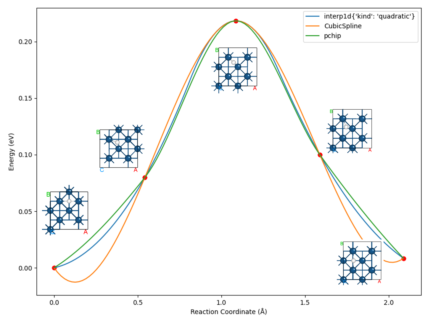
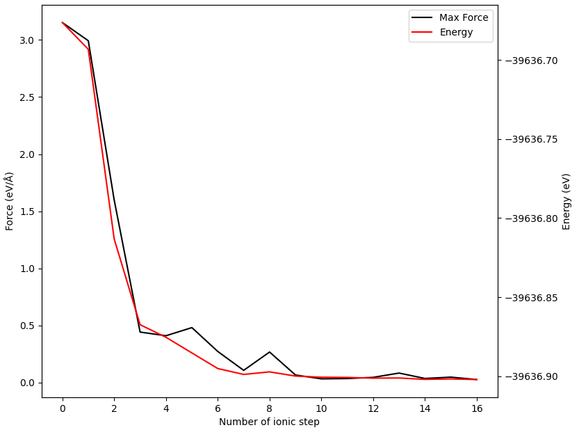
The energy and force of the 02 image obtained during the relaxation process are shown as follows:
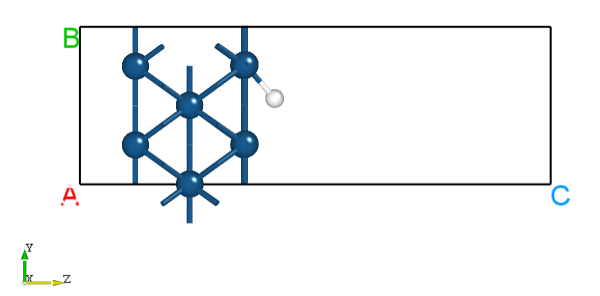
Alternatively, you can use the python script neb_movie.py to analyze the trajectory changes in the transition state search. The generated neb_movie.json file can be opened with Device Studio, and a frame is captured as shown below:
2.16 Phonon Dispersion Calculation
This section introduces how the DS-PAW code performs phonon calculations and computes phonon band structures and phonon density of states (DOS). DS-PAW supports two methods for phonon spectrum calculations: the finite displacement (fd) method and the density functional perturbation theory (DFPT) method. Taking a single MgO system as an example, this section explains how to calculate phonon bands and DOS using both methods, and analyzes the phonon band structure and DOS plots.
\(MgO\) Phonon Dispersion Calculation Input File
The input files consist of the parameter file phonon.in and the structure file structure.as. The phonon.in file is as follows:
 1task = phonon
 2
 3sys.structure = structure.as
 4sys.functional = PBE
 5sys.spin = none
 6
 7cal.methods = 1
 8cal.smearing = 1
 9sys.symmetry = true
10scf.convergence = 1.0e-07
11cal.ksamping = G
12cal.kpoints = [3,3,3]
13cal.sigma = 0.25
14
15phonon.type = bandDos
16phonon.structureSize = [2,2,2]
17phonon.primitiveUVW = [0.0, 0.5, 0.5, 0.5, 0.0, 0.5, 0.5, 0.5, 0.0]
18phonon.method = dfpt
19phonon.qpoints = [41,41,41]
20phonon.dosRange = [0,20]
21phonon.qpointsLabel = [G,X,W,G,M]
22phonon.qpointsCoord = [0.0, 0.0, 0.0, 0.5, 0.0, 0.0, 0.5, 0.5, 0.0, 0.0, 0.0, 0.0, 0.5, 0.5, 0.5]
23phonon.qpointsNumber = 51
24
25io.charge = false
26io.wave = false
phonon.in input parameter introduction:
In phonon calculations, you can generally retain the parameters of sys. and cal. in :guilabel:`phonon.in and then set the specific parameters for phonon calculations:
task: Sets the calculation type, which is phonon for this calculation;phonon.type: Set the type of phonon calculation, bandDos corresponds to calculating phonon band structure and density of states;phonon.structureSize: Set the size of the supercell for phonon calculations;phonon.primitiveUVW: Set the coefficients of the primitive cell UVW for phonon band calculations;phonon.method: Sets the method for phonon calculations, with “dfpt” indicating the Density Functional Perturbation Theory method;phonon.qpoints: Set the q-space grid sampling for phonon calculation to 41*41*41;phonon.dosRange: Sets the energy range for phonon density of states calculation to [0, 20];phonon.qpointsLabel: Set the labels for high-symmetry points in phonon band calculations;phonon.qpointsCoord: Set the coordinates of high-symmetry points for phonon band calculations.phonon.qpointsNumber: Set the interval between adjacent high-symmetry points for phonon band calculations;
The structure.as file is referenced as follows:
 1Total number of atoms
 28
 3Lattice
 4   4.2555564654942897    0.0000000000000000    0.0000000000000000
 5   0.0000000000000000    4.2555564654942888    0.0000000000000000
 6   0.0000000000000000    0.0000000000000000    4.2555564654942897
 7Direct
 8Mg  0.0000000000000000  0.0000000000000000  0.0000000000000000
 9Mg  0.0000000000000000  0.5000000000000000  0.5000000000000000
10Mg  0.5000000000000000  0.0000000000000000  0.5000000000000000
11Mg  0.5000000000000000  0.5000000000000000  0.0000000000000000
12O   0.5000000000000000  0.5000000000000000  0.5000000000000000
13O   0.5000000000000000  0.0000000000000000  0.0000000000000000
14O   0.0000000000000000  0.5000000000000000  0.0000000000000000
15O   0.0000000000000000  0.0000000000000000  0.5000000000000000
备注
When performing phonon calculations, the convergence accuracy of the self-consistent calculation should be increased; it is recommended to set it to 1.0e-7 or higher.
When performing phonon calculations with symmetry enabled, it is recommended to increase the accuracy of symmetry determination appropriately. The parameter sys.symmetryAccuracy can be set to 1.0e-6 or smaller to help obtain accurate calculation results.
phonon.iniPhonon can specify the path to read the phonon calculation (phonon.type = phonon) generated phonon.h5 file, enabling direct calculation of band structures and density of states.
phonon.type controls the type of phonon calculation. “phonon” corresponds to phonon calculation, “band” corresponds to phonon band calculation, “dos” corresponds to phonon density of states calculation, and “bandDos” corresponds to simultaneous calculation of phonon band and density of states. When phonon.type = band/dos/bandDos and no file path is specified for phonon.iniPhonon, the program first automatically performs the phonon calculation for phonon.type = phonon, and then calculates the band structure or density of states according to the task.
run program execution
After preparing the input files, upload the phonon.in and structure.as files to the server and run them, executing DS-PAW phonon.in as described in Structure Relaxation.
Analysis of Calculation Results
Based on the input files mentioned above, the calculation will generate the following output files: DS-PAW.log, phonon.h5, dfpt.json, and dfpt.as.
DS-PAW.log : The log file generated after the DS-PAW phonon calculation.
dfpt.as : Supercell structure file for phonon calculations, and this file is read during phonon calculations.
dfpt.json : Parameter file for phonon calculations, which is consistent with the information in the phonon.in file. This file is read when calculating phonons.
phonon.h5 : The h5 data file after the phonon calculation is completed; the phonon band data is stored in phonon.h5 at this point, and the specific data structure is detailed in the Output File Format Specification section;
You can use a python script to process the data in phonon.h5. The phonon band structure and density of states plots obtained after processing should look like (a) and (b) below:
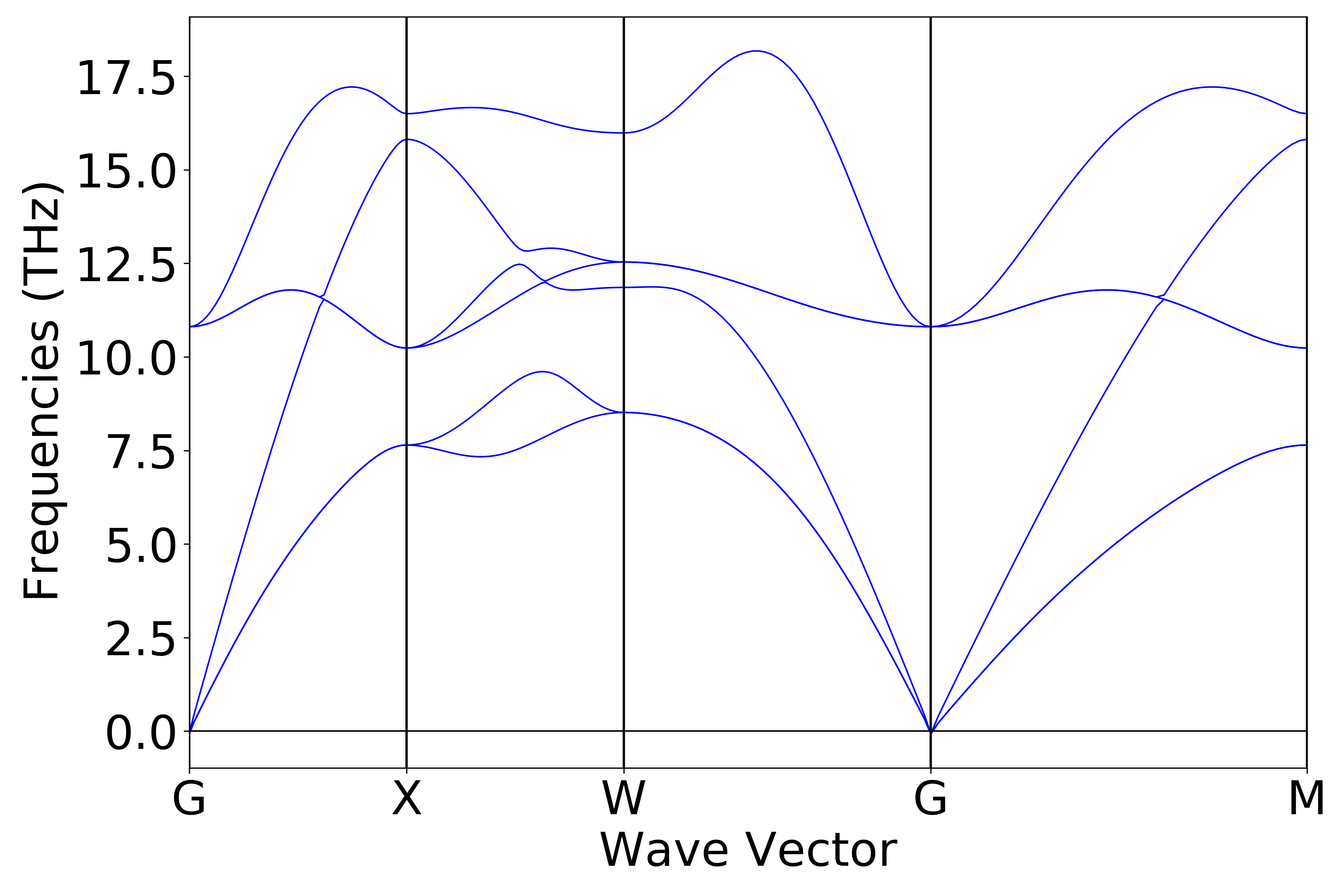
(a)
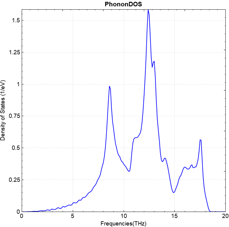
(b)
Analysis of NAC calculation results
The previous section presented the phonon band calculation without considering long-range interactions. To perform phonon calculations with the non-analytical term correction (nac), you can add the following two parameters to the phonon.in file shown in the previous section:
1phonon.dfptEpsilon=true
2phonon.nac = true
The resulting phonon band structure should look like (c) below:

(c)
fdphonon: Finite Displacement Method for Phonon Calculation
The input file for finite displacement (fd) phonon calculations is as follows. Simply modify the parameter phonon.method = dfpt to phonon.method = fd. Note that the output files generated by the fd method are different from those generated by the dfpt method.
 1task = phonon
 2
 3sys.structure = structure.as
 4sys.functional = PBE
 5sys.spin = none
 6
 7cal.methods = 1
 8cal.smearing = 1
 9sys.symmetry = true
10scf.convergence = 1.0e-07
11cal.ksamping = G
12cal.kpoints = [3,3,3]
13cal.sigma = 0.25
14
15phonon.type = bandDos
16phonon.structureSize = [2,2,2]
17phonon.primitiveUVW = [0.0, 0.5, 0.5, 0.5, 0.0, 0.5, 0.5, 0.5, 0.0]
18phonon.method = fd
19phonon.qpoints = [41,41,41]
20phonon.qpointsLabel = [G,X,W,G,M]
21phonon.qpointsCoord = [0.0, 0.0, 0.0, 0.5, 0.0, 0.0, 0.5, 0.5, 0.0, 0.0, 0.0, 0.0, 0.5, 0.5, 0.5]
22phonon.qpointsNumber = 51
23
24io.charge = false
25io.wave = false
For the MgO system, for example, when phonon.structureSize is set to [2,2,2], after the finite difference (FD) calculation is completed, two files, DS-PAW.log and phonon.h5, will be generated, along with folders 001 and 002. Folder 001 contains the files input.json and disp-001.as, and folder 002 contains input.json and disp-002.as. The two files in each subfolder are equivalent to the in file (input parameters) and the as file (structure parameters).
The number of generated folders (001, 002, …) depends on the symmetry of the system.
Using a python script to process the phonon.h5 file obtained from the finite displacement method calculation, the resulting band structure and density of states plots are consistent with plots (a) and (b) calculated using the dfpt method.
备注
The calculation of dielectric constant is only possible when phonon.method = dfpt.
The switch of phonon.nac is only effective when phonon.method = dfpt and phonon.dfptEpsilon=true
2.17 soc spin-orbit coupling calculation
This section describes how DS-PAW performs spin-orbit coupling calculations. Taking the \(Bi_{2}Se_{3}\) system as an example, we use a two-step method to calculate and analyze the band structure.
\(Bi_{2}Se_{3}\) Spin-Orbit Coupling Calculation Input File
First, a self-consistent calculation is performed: the input file contains the parameter file soi.in and the structure file structure.as, and soi.in is as follows:
 1# task type
 2task = scf
 3#system related
 4sys.structure = structure.as
 5sys.symmetry = false
 6sys.functional = PBE
 7#scf related
 8cal.methods = 2
 9cal.smearing = 1
10cal.ksamping = G
11cal.kpoints = [7, 7, 7]
12cal.cutoffFactor = 1.5
13#soi related
14sys.spin= non-collinear
15sys.soi = true
16#outputs
17io.charge = true
18io.wave = false
soi.in Input Parameter Description:
In spin-orbit coupling calculations, you can generally retain the parameters from sys. and cal. in the :guilabel:`soi.in file and then configure the specific parameters for the spin-orbit coupling calculation:
sys.spin: Sets the spin type of the system; non-collinear means non-collinear spin.sys.soi: Controls whether to consider spin-orbit coupling effect; this parameter is effective when sys.spin=non-collinear;
The following describes the structure.as file:
 1Total number of atoms
 25
 3Lattice
 4-2.069  -3.583614  0.000000
 52.069  -3.583614  0.000000
 60.000   2.389075  9.546667
 7Direct
 8Bi 0.3990 0.3990 0.6970
 9Bi 0.6010 0.6010 0.3030
10Se 0.0000 0.0000 0.5000
11Se 0.2060 0.2060 0.1180
12Se 0.7940 0.7940 0.8820
Input file for band structure calculation: soiband.in, content as follows
 1# task type
 2task = band
 3#system related
 4sys.structure = structure.as
 5sys.symmetry = true
 6sys.functional = PBE
 7#scf related
 8cal.methods = 2
 9cal.smearing = 1
10cal.ksamping = G
11cal.kpoints = [7, 7, 7]
12cal.cutoffFactor = 1.5
13#band related
14cal.iniCharge = ./rho.bin
15band.kpointsCoord = [0.00000000,0.00000000,0.00000000,0.00000000,0.00000000,0.50000000,0.50000000,0.50000000,0.00000000,0.00000000,0.00000000,0.00000000,0.50000000,0.00000000,0.00000000]
16band.kpointsLabel = [G,Z,F,G,L]
17band.kpointsNumber = [20,20,20,20]
18band.project = true
19#soi related
20sys.spin= non-collinear
21sys.soi = true
Introduction to input parameters in soiband.in:
In spin-orbit coupling band calculations, the parameters from the self-consistent calculation and spin-orbit coupling calculation are retained in soiband.in. After that, you can set the specific parameters for the band calculation.
备注
Initial magnetic moment setup refers to “Application Case - Antiferromagnetic Calculation of the NiO System”. Set the Mag tag on the seventh line of the structure.as file.
Run the program
After preparing the input files, upload the soi.in, soiband.in, and structure.as files to the server for execution. Run DS-PAW soi.in and DS-PAW soiband.in separately, following the methods described in the structural relaxation section.
Analysis Result Analysis
Based on the input files, after calculation completion, output files such as DS-PAW.log, scf.h5, and band.h5 will be generated.
The processing of band.h5 follows the same method as the band calculation described in Section 2.3. The resulting band structure should be as shown in Figure (a) below. Additionally, a calculation without spin-orbit coupling should yield the band structure shown in Figure (b) below:
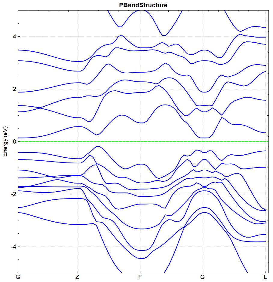
(a)
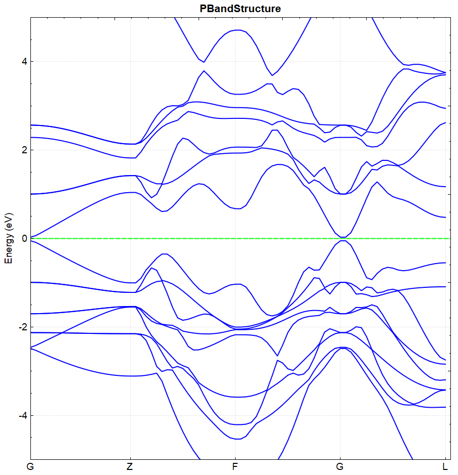
(b)
The BandGap values are read from DS-PAW.log. The band gap values for Figures (a) and (b) are 0.3251 eV and 0.0814 eV, respectively. This leads to the conclusion that spin-orbit coupling calculations increase the band gap between the valence and conduction bands.
2.18 AIMD molecular dynamics simulation
This section will introduce how to perform molecular dynamics simulations in DS-PAW, using a water molecule system as an example.
Input file for \(H_{2}O\) molecular dynamics simulation
The input files include the parameter file aimd.in and the structure file structure.as. aimd.in is shown below:
 1#task type
 2task = aimd
 3
 4#system related
 5sys.structure = structure.as
 6sys.symmetry = false
 7sys.functional = PBE
 8sys.spin = none
 9
10#scf related
11cal.methods = 1
12cal.smearing = 1
13cal.ksamping = G
14cal.kpoints = [1, 1, 1]
15cal.sigma = 0.1
16
17#aimd related
18aimd.ensemble = NPT
19aimd.thermostat = langevin
20aimd.atomFCoeffElements = [H_1]
21aimd.atomFCoeffs = [1]
22aimd.latticeFCoeff = 1
23aimd.pressure = 100
24aimd.timeStep = 1
25aimd.totalSteps = 2000
26aimd.iniTemp = 2000
27
28#outputs
29io.charge = false
30io.wave = false
aimd.in Input Parameters:
In the molecular dynamics simulation calculation, try to keep the parameters in sys. and cal. in aimd.in, then set the parameters specific to the molecular dynamics simulation calculation.
task: Sets the calculation type. In this case, the calculation is an AIMD molecular dynamics simulation.aimd.ensemble: Specifies the ensemble used for the molecular dynamics simulation. In this case, the ensemble is set to NPT.aimd.thermostat: Sets the thermostat or barostat used in the molecular dynamics simulation. In this example, the Langevin thermostat and barostat are used.aimd.atomFCoeffElements: Specifies the element names of the atoms considered as Langevin atoms. In this example, one hydrogen atom is set as a Langevin atom, and it is renamed to H_1;aimd.atomFCoeffs: Sets the friction coefficients for atoms considered as Langevin atoms, in units of ps-1;aimd.latticeFCoeff: Sets the friction coefficient of the lattice in the Langevin thermostat, unit ps-1;aimd.pressure: Sets the target pressure value for NPT simulations, in kbar;aimd.timeStep: Sets the time step for molecular dynamics simulation, in fs;aimd.totalSteps: Set the total number of steps for the molecular dynamics simulation;aimd.iniTemp: Sets the initial temperature for molecular dynamics simulations, in K;
The structure.as file is referenced as follows:
 1Total number of atoms
 23
 3Lattice
 44.00000000 0.00000000 0.00000000
 50.00000000 4.00000000 0.00000000
 60.00000000 0.00000000 4.00000000
 7Cartesian
 8H 2.63934013 1.89542007 1.58223984
 9H_1 1.36065987 2.11498988 2.45934006
10O 1.65002999 1.88501012 1.54065994
备注
The element renaming rule is “original element name + underscore + custom field.”
In this example, the second hydrogen atom is set as a Langevin atom and renamed to H_1. The element name for this atom needs to be manually modified in the structure.as file.
Since a custom element name H_1 exists in the calculation system, the program will automatically search for the pseudopotential of the corresponding H element for H_1, and the user does not need to prepare a new pseudopotential.
run the program
Once the input files are prepared, upload the files aimd.in and structure.as to the server and run them. Execute DS-PAW aimd.in as described in Structure Relaxation.
Analysis of calculation results.
Based on the input files mentioned above, the calculation will produce output files such as DS-PAW.log, aimd.h5, and latestStructure.as upon completion.
DS-PAW.log : Log file generated by the DS-PAW molecular dynamics simulation.
aimd.h5 : The h5 output file corresponding to the molecular dynamics calculation; atom positions, system energy, temperature, and other data during the simulation are saved in aimd.h5. For details on the data structure, see the Output File Format Specification section.
latestStructure.as : The final state as structure file from molecular dynamics simulation, storing the final configuration and velocity information;
Data processing of the aimd.h5 file can be performed using a python script, as detailed in the Auxiliary Tool User Guide section. The following figures should show the pressure vs. time and temperature vs. time curves obtained from a 2000-step NPT ensemble simulation:
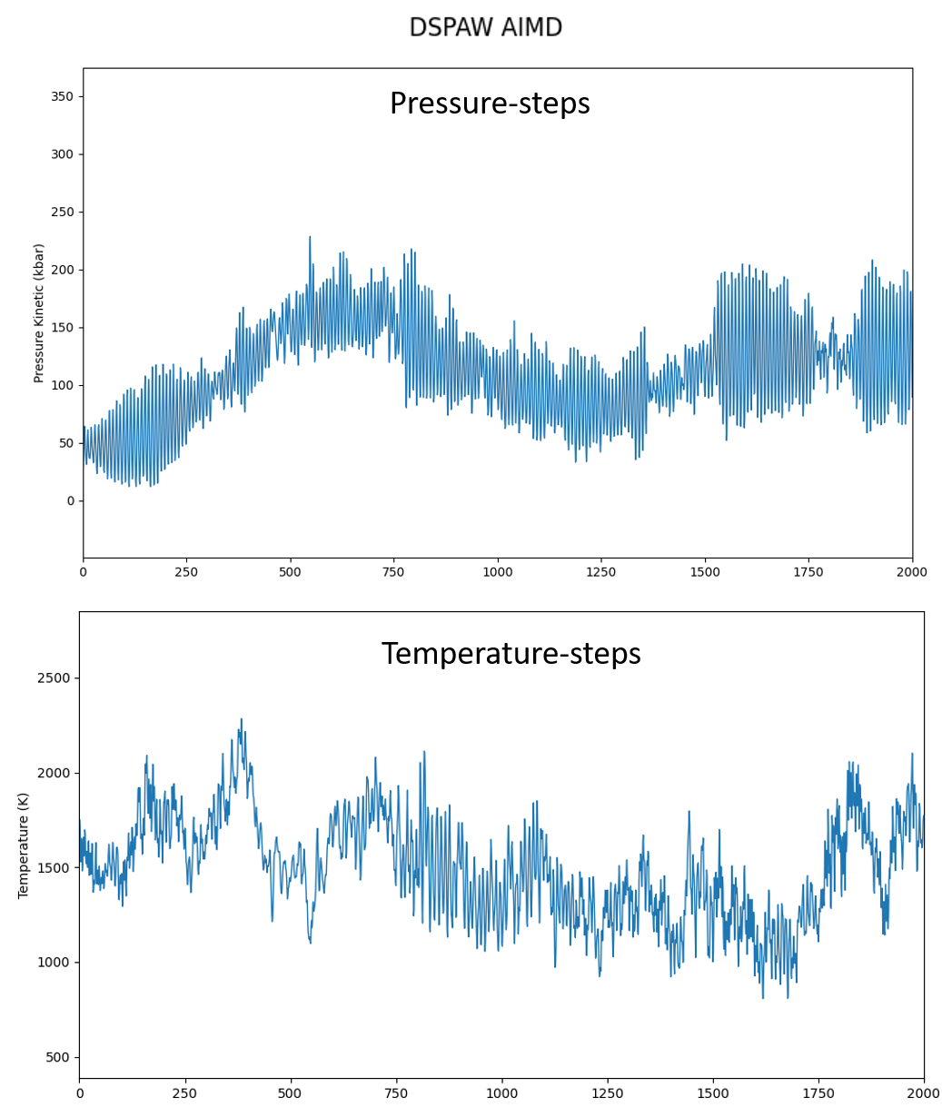
备注
Different ensembles correspond to different optional thermostat ranges: the NVE ensemble can choose the Andersen thermostat; the NVT ensemble can choose the Andersen, Nose-Hoover, and Langevin thermostats; the NPT and NPH ensembles can choose the Langevin thermostat.
To simulate a high-temperature annealing process, set `aimd.ensemble` to SA and set the initial and final temperatures via `aimd.iniTemp` and `aimd.finTemp` respectively.
The parameter `aimd.finTemp` only takes effect during simulated annealing. For constant-temperature ensembles such as NPT and NVT, the final temperature is equal to the initial temperature.
When simulating a system containing langevin atoms, it is recommended to store the pseudopotential files corresponding to the langevin atoms in the calculation directory to avoid the program reporting error E3058 due to failure to find the pseudopotential files.
2.19 efield plus applied electric field calculation
This section will use the band calculation of a silicene model as an example to demonstrate how to perform calculations with an external electric field in DS-PAW, and analyze the band gap opening before and after applying the electric field.
Input file for silicene calculation with external electric field in vacuum
The input file contains parameter file Efield.in and structure file structure.as, Efield.in is as follows:
 1# task type
 2task = scf
 3#system related
 4sys.structure = structure.as
 5sys.symmetry = true
 6sys.functional = PBE
 7sys.spin = none
 8
 9#scf related
10cal.sigma = 0.1
11cal.cutoff = 520
12cal.ksamping = G
13cal.kpoints = [9, 9, 1]
14
15scf.convergence = 1e-5
16
17#outputs
18io.charge = false
19io.wave = false
20io.band = true
21
22corr.dipol=true
23corr.dipolDirection = c
24corr.dipolEfield = 0.2
25
26band.kpointsLabel = [G,M,K,G]
27band.kpointsCoord = [0.00000000,0.00000000,0.00000000,0.50000000,0.00000000,0.00000000,0.33333333,0.33333333,0.00000000,0.00000000,0.00000000,0.00000000]
28band.kpointsNumber = [100,100,100]
Efield.in Input Parameters:
The calculation is performed on top of a one-step band calculation with an external electric field. In addition to the basic parameters of the band calculation, the following new parameters are introduced:
corr.dipolEfield: Sets the magnitude of the applied electric field. This parameter is only effective whencorr.dipol = trueandcorr.dipolDirectionis set;
The structure.as file is referenced as follows:
1Total number of atoms
22
3Lattice
43.860000   0.000000   0.000000
5-1.930000   3.342860   0.000000
60.000000   0.000000  26.460000
7Direct
8Si   0.333333   0.166667   0.396825
9Si   0.666758   0.833380   0.379216
run program execution
After preparing the input files, upload the Efield.in and structure.as files to the server for execution, and run DS-PAW Efield.in as described in the structure relaxation section.
Analysis of calculation results
Based on the input files mentioned above, the calculation will generate output files such as DS-PAW.log and scf.h5.
:guilabel:`scf.h5: The h5 output file corresponding to the self-consistent field (SCF) calculation. When io.band = true, the band structure data will be written to the scf.h5 file;
In this example, the parameter corr.dipolEfield = 0.2, indicating an applied electric field strength of 0.2 eV/Å. The band structure calculated under this electric field is shown in Figure (a).
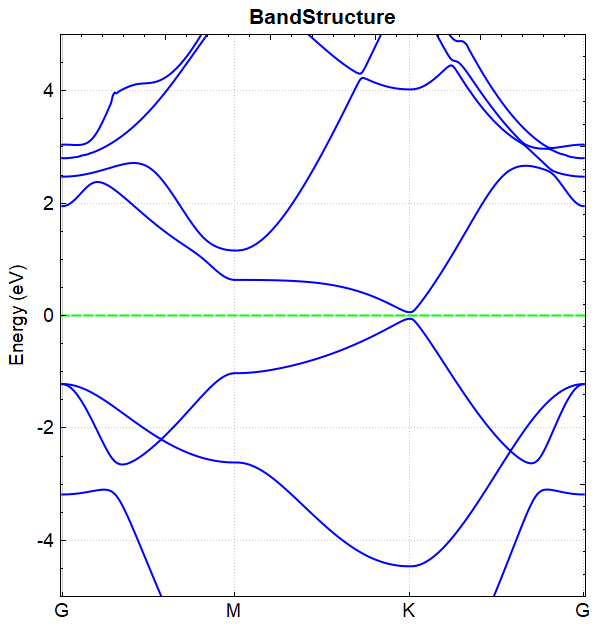
(a)
Repeating the above calculation with the parameter corr.dipolEfield = 0, i.e., band structure calculation without an electric field, results in the band diagram shown in Figure (b).
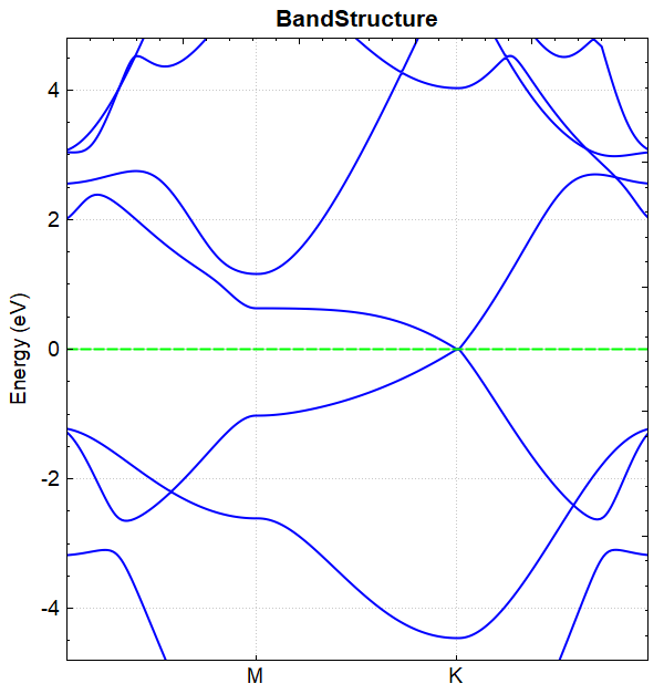
(b)
Comparing figures (a) and (b), we can conclude that applying an external electric field can open the band gap of silicene. The values of the BandGap with and without the electric field, readable from the DS-PAW.log file, are 0.1176 eV and 0.0010 eV, respectively.
备注
The unit of the external electric field, eV/Å, is also the unit of atomic force.
2.20 polarization ferroelectric calculation
This section will use \(HfO_{2}\) as an example to introduce how to perform ferroelectric calculations using modern polarization theory in DS-PAW, analyzing the ferroelectric polarization of \(HfO_{2}\).
\(HfO_{2}\) Ferroelectric Calculation Input File
The input files include the parameter file polarization.in and a series of structure files for different phases structure.as. The contents of polarization.in are as follows:
 1# task type
 2task = scf
 3#system related
 4sys.structure = structure.as
 5sys.symmetry = true
 6sys.functional = PBE
 7sys.spin = none
 8
 9#scf related
10cal.methods = 3
11cal.smearing = 4
12cal.cutoff = 520
13cal.ksamping = MP
14cal.kpoints = [4, 4, 4]
15
16scf.convergence = 1e-5
17
18#outputs
19io.charge = false
20io.wave = false
21io.polarization = true
:guilabel:`polarization.in Input Parameters:`
This calculation performs ferroelectric calculations based on a self-consistent calculation. In addition to the basic parameters for the self-consistent calculation, the following parameters are newly added:
io.polarization: Controls the switch for ferroelectric calculations in the self-consistent calculation;
The following is a reference structure.as file for the ferroelectric phase structure of \(HfO_{2}\) with polarization pointing downwards:
 1Total number of atoms
 212
 3Lattice
 45.04621935 0.00000000 0.00000000
 50.00000000 5.07315250 0.00000000
 60.00000000 0.00000000 5.25768906
 7Cartesian
 8Hf 1.34815269 1.22145222 0.17639072
 9Hf 1.34815269 3.75802848 2.45245381
10Hf 3.69806665 1.22145222 2.80523525
11Hf 3.69806665 3.75802848 5.08129834
12O 0.35195212 1.93667284 1.92589951
13O 0.35195212 4.47324910 0.70294502
14O 2.32678304 2.48829365 3.85528783
15O 2.32678304 5.02486989 4.03124575
16O 2.71943629 5.02486989 1.40240122
17O 2.71943629 2.48829365 1.22644331
18O 4.69426723 1.93667284 4.55474404
19O 4.69426723 4.47324910 3.33178954
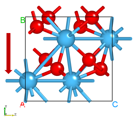
\(HfO_{2}\) ferroelectric phase structure with polarization pointing upwards, see the structure.as file below:
 1Total number of atoms
 212
 3Lattice
 45.04621935 0.00000000 0.00000000
 50.00000000 5.07315250 0.00000000
 60.00000000 0.00000000 5.25768906
 7Cartesian
 8Hf 1.34815269 1.31512402 0.17639072
 9Hf 1.34815269 3.85170026 2.45245381
10Hf 3.69806665 1.31512402 2.80523525
11Hf 3.69806665 3.85170026 5.08129834
12O 0.35195212 0.59990340 1.92589951
13O 0.35195212 3.13647965 0.70294502
14O 2.32678304 2.58485884 4.03124575
15O 2.32678304 5.12143510 3.85528783
16O 2.71943630 5.12143510 1.22644331
17O 2.71943630 2.58485884 1.40240122
18O 4.69426723 0.59990340 4.55474404
19O 4.69426723 3.13647965 3.33178954
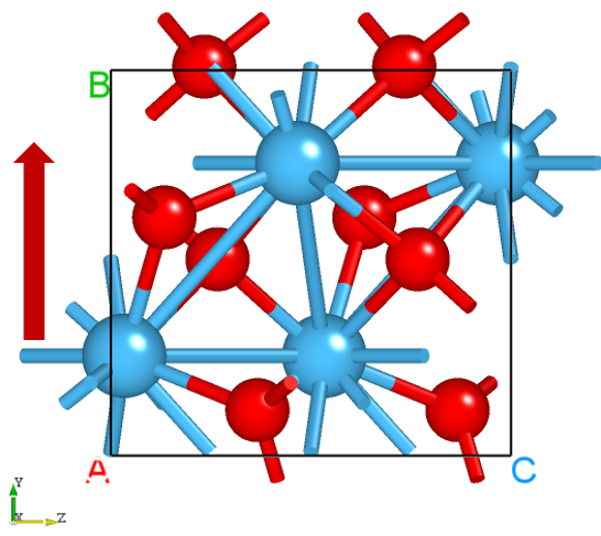
Insert a series of intermediate transition structures between the polarization-down and polarization-up structures using linear interpolation (neb.linear_interpolate), as detailed in the utility script neb_structure.py. In this example, 11 intermediate structures are inserted, resulting in a total of 13 configurations including the initial and final polarization phases. Polarization calculations are then performed sequentially on all configurations.
Run the program.
After preparing the input files, upload polarization.in and each structure.as file to the server, placing the 13 structures into 13 directories. Then, execute DS-PAW polarization.in following the method described in Structure Relaxation.
Analysis of calculation results
Based on the input files mentioned above, 13 sets of output files will be generated after the calculation, including DS-PAW.log, scf.h5, and polarization.txt.
DS-PAW.log : The log file generated after the DS-PAW ferroelectric calculation.
scf.h5 : The self-consistent field (SCF) calculation output file in h5 format. Note that the name of the h5 file must strictly match the task type. For h5 file parsing, refer to the Output File Format Specification section.
polarization.txt : The txt file generated after the ferroelectric polarization calculation is completed. It stores the electronic and ionic contributions to polarization, as well as the total polarization quantum number, for easy access by the user.
For the ferroelectric phase system with downward polarization (00) as an example, the ferroelectric polarization data of \(HfO_{2}\) can be obtained from the polarization.txt file as follows:
Total(x y z) ( \(\mu C/cm^2\) )
-0.000043
-8.715604
-0.000002
Quantum(x y z) ( \(\mu C/cm^2\) )
60.067225
60.387821
62.584436
For example, in a polarization-up (12) ferroelectric phase system, the ferroelectric polarization data for \(HfO_{2}\) can be obtained from the polarization.txt file as follows:
Total(x y z) ( \(\mu C/cm^2\) )
-0.000049
8.715446
0.000001
Quantum(x y z) ( \(\mu C/cm^2\) )
60.067225
60.387821
62.584436
The PolaTotal.py script can be used to process the scf.h5 file that writes polarization data. See the Auxiliary Tool User Guide section for specific instructions. Processing the data for 13 ferroelectric calculations yields the following result figure:
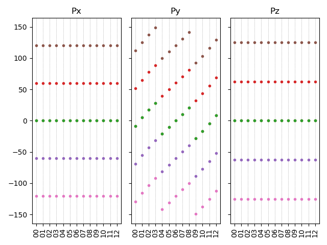
The figure above shows the polarization intensity Px, Py, and Pz in the x, y, and z directions, obtained after polarization quantum periodic conversion. Since the polarization direction of \(HfO_{2}\) is the y-direction, the values of Px and Pz do not change with atomic displacement.
Analyzing the group with the polarization number closest to 0 in the Py direction, the polarization intensity value of \(HfO_{2}\) is the difference in polarization number between the ferroelectric phase (downward polarization, sequence number 00 or upward polarization, sequence number 12) and the central symmetric phase (transition state, sequence number 06), combined with the polarization.txt file and the polarization data figure above, to obtain:
The polarization difference between configurations 00 and 06 is \(-69.103 \mu C/cm^2\)
The polarization difference between configurations 12 and 06 is \(69.103 \mu C/cm^2\)
Therefore, the polarization intensity of \(HfO_{2}\) is \(69.103\mu C/cm^2\)
2.21 Bader Charge Calculation
This section will use the NaCl crystal as an example to introduce how to perform Bader charge calculation in DS-PAW and analyze the valence distribution of each atom in the NaCl system.
Input file for Bader charge calculation of \(NaCl\) crystal
The input files include the parameter file bader.in and the structure file structure.as. bader.in is as follows:
The bader.in file is shown below:
 1# task type
 2task = scf
 3#system related
 4sys.structure = structure.as
 5sys.symmetry = true
 6sys.functional = PBE
 7sys.spin = none
 8
 9#scf related
10cal.methods = 1
11cal.smearing = 1
12cal.ksamping = G
13cal.kpoints = [10, 10, 10]
14cal.cutoff = 650
15#outputs
16io.charge = true
17io.wave = false
18io.bader = true
bader.in Input Parameter Description:
This Bader charge calculation is performed based on the self-consistent calculation. In addition to the basic parameters of the self-consistent calculation, the following new parameters are added:
io.bader: Controls the Bader charge calculation switch during the self-consistent calculation;
The structure.as file is referenced as follows:
 1Total number of atoms
 28
 3Lattice
 45.68452692 0.00000000 0.00000000
 50.00000000 5.68452692 0.00000000
 60.00000000 0.00000000 5.68452692
 7Cartesian
 8Na 4.26339519 1.42113173 1.42113173
 9Na 1.42113173 4.26339519 1.42113173
10Na 1.42113173 1.42113173 4.26339519
11Na 4.26339519 4.26339519 4.26339519
12Cl 1.42113173 1.42113173 1.42113173
13Cl 4.26339519 4.26339519 1.42113173
14Cl 4.26339519 1.42113173 4.26339519
15Cl 1.42113173 4.26339519 4.26339519
备注
When io.bader is true, io.charge must also be true.
Run the program
After preparing the input files, upload the bader.in and structure.as files to the server for execution. Run DS-PAW bader.in following the methods described in the structural relaxation section.
Analysis results analysis
Based on the input files mentioned above, after the calculation is complete, output files such as DS-PAW.log, scf.h5, and bader.txt will be generated.
DS-PAW.log : The log file generated after the DS-PAW Bader charge calculation.
scf.h5 : The self-consistent field (SCF) calculation output file in h5 format. Note that the name of the h5 file must strictly match the task type. For h5 file parsing, see the specific data structure details in the Output File Format Specification section;
bader.txt : The txt file generated after the Bader charge calculation, containing Bader charge data for quick access by users.
The content of the bader.txt file is as follows, and the data obtained from the Bader charge analysis is consistent with the data from the Henkelman group at the University of Texas at Austin.
Total number of valence electronics: 64
Element |
X |
Y |
Z |
Charge |
AtomicVolume |
MinDistance |
Cl |
0.25 |
0.25 |
0.25 |
7.85852 |
35.893 |
1.65799 |
Cl |
0.75 |
0.75 |
0.25 |
7.85704 |
35.83 |
1.65799 |
Cl |
0.75 |
0.25 |
0.75 |
7.84024 |
35.0495 |
1.65799 |
Cl |
0.25 |
0.75 |
0.75 |
7.87537 |
36.6765 |
1.65799 |
Na |
0.75 |
0.25 |
0.25 |
8.14221 |
10.0598 |
1.10532 |
Na |
0.25 |
0.75 |
0.25 |
8.14223 |
10.0607 |
1.10532 |
Na |
0.25 |
0.25 |
0.75 |
8.14221 |
10.0598 |
1.10532 |
Na |
0.75 |
0.75 |
0.75 |
8.14221 |
10.0598 |
1.10532 |
2.22 bandunfolding calculation
This section will use the \(Cu_{3}Au\) system as an example to demonstrate how to perform band unfolding calculations in DS-PAW, and analyze the band structure of \(Cu_{3}Au\) after unfolding.
\(Cu_{3}Au\) band unfolding calculation input file
Band unfolding calculations require a two-step band calculation. Therefore, the input files include the parameter files scf.in, bandunfolding.in, and the structure file structure.as.
The scf.in file is as follows:
 1task = scf
 2
 3sys.structure = structure.as
 4sys.symmetry = true
 5sys.functional = PBE
 6sys.spin = none
 7
 8cal.methods = 1
 9cal.smearing = 1
10cal.ksamping = MP
11cal.kpoints = [3, 3, 3]
12cal.cutoff = 650
13
14scf.convergence = 1.0e-05
15
16io.charge = true
17io.wave = false
bandunfolding.in as follows:
 1task = band
 2cal.iniCharge = ./rho.bin
 3
 4sys.structure = structure.as
 5sys.symmetry = true
 6sys.functional = PBE
 7sys.spin = none
 8
 9cal.methods = 1
10cal.smearing = 1
11cal.ksamping = MP
12cal.kpoints = [3, 3, 3]
13cal.cutoff = 500
14
15scf.convergence = 1.0e-05
16
17band.unfolding = true
18band.primitiveUVW=[0.0, 0.5, 0.5, 0.5, 0.0, 0.5, 0.5, 0.5, 0.0]
19band.kpointsLabel= [R,G,X]
20band.kpointsCoord= [0.5, 0.5, 0.5, 0.0, 0.0, 0.0, 0.5, 0.0, 0.5]
21band.kpointsNumber= [101, 101]
22
23io.charge = false
24io.wave = false
bandunfolding.in Input parameter introduction:
The band unfolding calculation is performed based on the band calculation, and the band calculation must be completed in a two-step process. In addition to the basic parameters for band calculation, the new parameters are as follows:
band.unfolding: Controls the switch for band unfolding calculation in band structure calculations;band.primitiveUVW: Sets the UVW coefficients. Multiplying the supercell lattice vectors by the UVW coefficients results in the primitive cell lattice vectors, which is used to control the band unfolding parameters.
The structure.as file is referenced as follows:
 1Total number of atoms
 24
 3Lattice
 43.7530000210         0.0000000000         0.0000000000
 50.0000000000         3.7530000210         0.0000000000
 60.0000000000         0.0000000000         3.7530000210
 7Direct
 8Au     0.000000000         0.000000000         0.000000000
 9Cu     0.000000000         0.500000000         0.500000000
10Cu     0.500000000         0.000000000         0.500000000
11Cu     0.500000000         0.500000000         0.000000000
run program execution
After preparing the input files, upload the scf.in, bandunfolding.in, and structure.as files to the server and run them. Execute DS-PAW scf.in as described in the structure relaxation section. After the self-consistent calculation is completed, execute DS-PAW bandunfolding.in.
Analysis of calculation results.
Based on the input files mentioned above, the calculation will generate output files such as DS-PAW.log, scf.h5, and band.h5.
:guilabel:`band.h5 : The h5 output file corresponding to the band structure calculation. Compared to the band structure calculation, this file adds the UnfoldingBandInfo section. See Output File Format Specification for a detailed structure analysis.
The script bandunfolding.py can be used to process data from band.h5. See Auxiliary Tool User Guide for detailed instructions. The resulting band structure plot should look like the following figure, consistent with the results reported in [1].
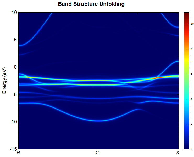
2.23 epsilon Dielectric Constant Calculation
This section will use the Si system as an example to introduce how to perform dielectric constant calculations in DS-PAW.
\(Si\) dielectric constant calculation input file
The input files consist of the parameter file epsilon.in and the structure file structure.as. The contents of epsilon.in are as follows:
 1# task type
 2task = epsilon
 3#system related
 4sys.structure = structure.as
 5sys.symmetry = true
 6sys.functional = PBE
 7sys.spin = none
 8
 9#scf related
10cal.methods = 1
11cal.smearing = 1
12cal.ksamping = G
13cal.kpoints = [5, 5, 5]
14cal.cutoff = 500
15scf.convergence = 1.0e-7
epsilon.in Input parameter introduction:
The calculation of dielectric constants can be performed by directly specifying task. The new optional values for task are as follows:
task: Sets the calculation type. Adds the epsilon parameter, which corresponds to the calculation of the dielectric constant here.
备注
Dielectric constant calculations are also possible when task = phonon and phonon.method = dfpt by adding the parameter phonon.dfptEpsilon = true.
The structure.as file is referenced as follows:
 1Total number of atoms
 28
 3Lattice
 4   5.43070000 0.00000000 0.00000000
 5   0.00000000 5.43070000 0.00000000
 6   0.00000000 0.00000000 5.43070000
 7Cartesian
 8Si 0.67883750 0.67883750 0.67883750
 9Si 3.39418750 3.39418750 0.67883750
10Si 3.39418750 0.67883750 3.39418750
11Si 0.67883750 3.39418750 3.39418750
12Si 2.03651250 2.03651250 2.03651250
13Si 4.75186250 4.75186250 2.03651250
14Si 4.75186250 2.03651250 4.75186250
15Si 2.03651250 4.75186250 4.75186250
run program execution
Once the input files are ready, upload the epsilon.in and structure.as files to the server and run the DS-PAW epsilon.in as described in the structure relaxation section.
Analysis of calculation results
Based on the input files mentioned above, the calculation will generate output files such as DS-PAW.log, epsilon.h5, and epsilon.txt.
DS-PAW.log : The log file generated after the DS-PAW dielectric constant calculation;
epsilon.h5 : The h5 output file corresponding to the dielectric constant calculation. For the specific data structure, see the Output File Format Specification section;
epsilon.txt : The txt text file generated after the dielectric constant calculation, which writes data related to the dielectric constant for quick user access.
The following data can be obtained from the epsilon.txt file:
Total Part |
||
13.309902 |
0.000000 |
-0.000000 |
-0.000000 |
13.309902 |
-0.000000 |
-0.000000 |
0.000000 |
13.309902 |
Analyzing the table above, the dielectric constant of the system is 13.309902, which is consistent with the literature value of 13.31 reported in :footcite:p:PhysRevB.73.045112.
2.24 Piezoelectric Tensor Calculation
This section will demonstrate how to calculate the piezoelectric tensor, specifically obtaining the piezoelectric coefficient \(e_{33} (0)\) for a material, using AlN as an example within the DS-PAW framework.
Input file for piezoelectric tensor calculation of \(AlN\)
The input file contains the parameter file piezo.in and the structure file structure.as, with piezo.in as follows:
 1task = epsilon
 2#system related
 3sys.structure = structure.as
 4sys.symmetry = true
 5sys.functional = PBE
 6sys.spin = none
 7
 8#scf related
 9cal.methods = 1
10cal.smearing = 1
11cal.ksamping = G
12cal.kpoints = [10, 10, 10]
13cal.cutoffFactor = 1.5
14scf.convergence = 1.0e-7
15
16#outputs
17io.charge = false
18io.wave = false
piezo.in Input parameter introduction:
task: Sets the calculation type, adding the epsilon parameter; here, it corresponds to the piezoelectric tensor calculation.scf.convergence: Sets the precision for electronic convergence in dielectric tensor calculations; it is recommended to increase the precision, which is set to 1.0e-7 here.
structure.as file is referenced as follows:
 1Total number of atoms
 28
 3Lattice
 43.11606630 0.00000000 0.00000000
 50.00000000 5.39683518 0.00000000
 60.00000000 0.00000000 5.00770902
 7Cartesian
 8Al 0.00000000 3.59735137 0.00946380
 9Al 0.00000000 1.79945276 2.51320124
10Al 1.55803315 0.89899597 0.00945662
11Al 1.55803315 4.49786165 2.51308138
12N 0.00000000 3.59851112 1.91845914
13N 0.00000000 1.79831356 4.42266820
14N 1.55803315 0.90013952 1.91851680
15N 1.55803315 4.49672497 4.42258192
run program execution
Once the input files are ready, upload the files piezo.in and structure.as to the server and run DS-PAW piezo.in following the method described in Structure Relaxation.
Analysis of calculation results
Based on the input files mentioned above, the calculation will produce the following output files: DS-PAW.log, epsilon.h5, and epsilon.txt.
DS-PAW.log : The log file generated after the DS-PAW piezoelectric tensor calculation.
epsilon.h5 : The h5 output file corresponding to the dielectric constant calculation, and the specific data structure can be found in the Output File Format Specification section;
epsilon.txt : The txt text file after the piezoelectric calculation is completed. This file writes piezoelectric-related data for users to quickly obtain information.
The following data can be obtained from the epsilon.txt file:
Piezoelectric Tensor (C/m^2)( Row: x y z Column: XX YY ZZ XY YZ ZX) |
|||||
Electronic Part |
|||||
0.000000 |
0.000000 |
0.000000 |
0.000006 |
0.000000 |
0.336610 |
-0.000001 |
0.000007 |
0.000003 |
0.000000 |
0.336662 |
0.000000 |
0.266339 |
0.265888 |
-0.419569 |
0.000000 |
-0.000014 |
0.000000 |
Ionic Part: |
|||||
-0.000004 |
0.000002 |
0.000002 |
0.000032 |
-0.000000 |
-0.681702 |
-0.000163 |
-0.000239 |
0.000314 |
-0.000000 |
-0.699012 |
-0.000000 |
-0.911456 |
-0.913265 |
1.943887 |
-0.000000 |
-0.000633 |
-0.000000 |
Total Part: |
|||||
-0.000004 |
0.000002 |
0.000002 |
0.000039 |
-0.000000 |
-0.345092 |
-0.000164 |
-0.000232 |
0.000317 |
-0.000000 |
-0.362350 |
-0.000000 |
-0.645117 |
-0.647377 |
1.524318 |
-0.000000 |
-0.000647 |
-0.000000 |
Analyzing the above table, the value of the piezoelectric tensor electronic contribution \(e_{33} (0)\) is -0.419569 \(C/m^{2}\), and the total piezoelectric tensor \(e_{33}\) is 1.524318 \(C/m^{2}\), which is close to the literature values[2] of -0.47 \(C/m^{2}\) and 1.46 \(C/m^{2}\).
2.25 fixcell Fixed Basis Vector Relaxation Calculation
This section will use the \(MoS_{2}\) system as an example to introduce how to perform fixed-lattice relaxation calculations in DS-PAW.
Fixed-basis-vector relaxation calculation input file for \(MoS_{2}\)
The input file consists of the parameter file relax.in and the structure file structure.as, with relax.in as follows:
 1# task type
 2task = relax
 3#system related
 4sys.structure = structure.as
 5sys.symmetry = false
 6sys.functional = PBE
 7sys.spin = none
 8
 9#scf related
10cal.methods = 1
11cal.smearing = 1
12cal.ksamping = G
13cal.cutoff = 650
14cal.kpoints = [19, 19, 5]
15#relax related
16relax.freedom = all
17relax.convergence =  0.05
18relax.methods = CG
The structure.as file is referenced as follows:
 1Total number of atoms
 26
 3Lattice  Fix_x Fix_y Fix_z
 43.19031572 0.00000000 0.00000000   F T T
 5-1.59515786 2.76289446 0.00000000  F F T
 60.00000000 0.00000000 14.87900448  T T T
 7Cartesian
 8S 0.00000000 1.84193052 12.72413785
 9S 1.59515943 0.92096386 5.28463561
10S 0.00000000 1.84193052 9.59436887
11S 1.59515943 0.92096386 2.15486663
12Mo 1.59515943 0.92096386 11.15925336
13Mo 0.00000000 1.84193052 3.71975112
Introduction to the structure.as tag settings:
To perform relaxation calculations with fixed cell dimensions, you need to add the fix tags in the structure.as file, similar to the fix tag settings for atomic relaxation (adding the Fix tag after the atomic coordinates). To fix the lattice vectors, add the Fix tag after the Lattice line on the third line of the structure.as file. In this case, the tags correspond to fixing the c-axis and the y and z directions of the a-axis, and the z direction of the b-axis of the cell.
Run the program.
After preparing the input files, upload the relax.in and structure.as files to the server and run them, executing DS-PAW relax.in as described in the structure relaxation section.
Analysis of calculation results
Based on the input files mentioned above, after the calculation is completed, output files such as DS-PAW.log, relax.h5, and latestStructure.as will be generated.
relax.h5: The corresponding h5 output file for the relaxation calculation;
latestStructure.as: The final structure file in .as format after relaxation, allowing direct data viewing;
Drag latestStructure.as into Device Studio to view the structure, or open the file directly to see the structural data after relaxation ends, as follows:
 1Total number of atoms
 26
 3Lattice
 43.19696732   0.00000000   0.00000000
 5-1.59848077   2.76865753   0.00000000
 60.00000000   0.00000000  14.87900448
 7Direct
 8Mo   0.66666701   0.33333316   0.74999995
 9Mo   0.33333340   0.66666675   0.24999997
10S   0.33333340   0.66666666   0.85535854
11S   0.66666686   0.33333303   0.35535875
12S   0.33333367   0.66666699   0.64464148
13S   0.66666708   0.33333333   0.14464130
Comparing the results, before relaxation a = b = 3.19031572, after relaxation a = b = 3.19696732, while c = 14.87900448 remained unchanged.
2.26 Calculation of Thermodynamic Properties of Phonons for Thermal Transport
This section will use a Si system as an example to introduce how to perform phonon thermodynamic property calculations in DS-PAW.
Input file for phonon thermodynamic properties calculation of \(Si\)
The input files include a parameter file, phonon-thermal.in, and a structure file, structure.as. phonon-thermal.in is shown below:
 1# task type
 2task = phonon
 3#system related
 4sys.structure = structure.as
 5sys.symmetry = true
 6sys.functional = PBE
 7sys.spin = none
 8
 9#scf related
10cal.methods = 1
11cal.smearing = 1
12cal.ksamping = G
13cal.kpoints = [5, 5, 5]
14cal.cutoffFactor = 1.5
15scf.convergence = 1.0e-7
16#phonon related
17phonon.structureSize = [2,2,2]
18phonon.type =dos
19phonon.qpoints = [31,31,31]
20phonon.method = dfpt
21
22phonon.thermal=true
23phonon.thermalRange = [0,1000,10]
Input parameters description for phonon-thermal.in:
phonon.thermal: Controls the thermodynamic calculation switch in phonon calculations; effective only when phonon.method = dfpt.phonon.thermalRange: Sets the temperature range and data storage interval for thermodynamic calculations;
The following describes the structure.as file:
1Total number of atoms
22
3Lattice
40.00 2.75 2.75
52.75 0.00 2.75
62.75 2.75 0.00
7Direct
8Si -0.125000000 -0.125000000 -0.125000000
9Si 0.125000000 0.125000000 0.125000000
Run the program
After preparing the input files, upload the phonon-thermal.in and structure.as files to the server for execution. Run DS-PAW phonon-thermal.in following the method described in the structural relaxation section.
Results Analysis
Based on the input files mentioned above, after the calculation is complete, output files such as DS-PAW.log and phonon.h5 will be generated.
DS-PAW.log: The log file generated from the DS-PAW phonon calculation.
phonon.h5: The h5 output file from the DS-PAW phonon calculation. Enabling thermodynamic calculations will write ThermalInfo data to the generated phonon.h5 file. See Output File Format Specification for details.
The phonon thermodynamic data can be processed using the phonon_thermal.py script, as detailed in the Auxiliary Tool User Guide section. Analyzing the thermodynamic data yields curves of entropy, heat capacity, and Helmholtz free energy as a function of temperature, which are consistent with the results presented in the phonopy git repository:
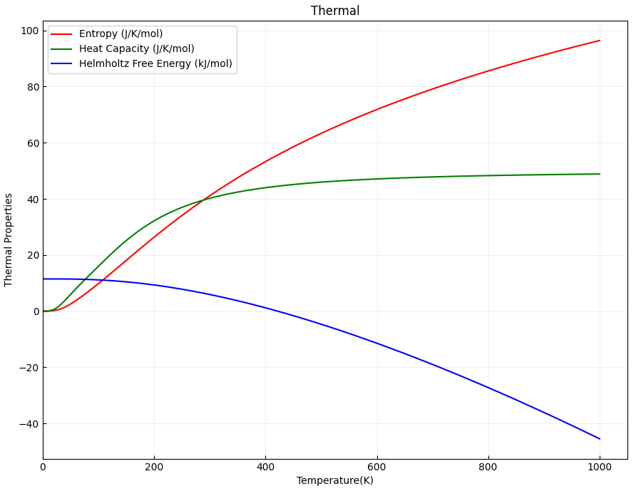
2.27 solid state NEB calculation
This section will use the HfZrO system as an example to illustrate how to perform solid state NEB calculations with cell relaxation within DS-PAW.
\(HfZrO\) Solid state NEB input file
The input files include the parameter file ssneb.in and the structure file structure.as, with the contents of ssneb.in as follows:
 1task = neb
 2
 3sys.structure = structure.as
 4sys.functional  = LDA
 5sys.spin = none
 6sys.symmetry = false
 7
 8cal.ksamping = G
 9cal.kpoints = [10,10,10]
10cal.cutoff = 650
11cal.methods = 1
12cal.smearing = 1
13cal.sigma = 0.05
14
15scf.mixType = Broyden
16scf.mixBeta = 0.4
17scf.convergence = 1e-6
18scf.max = 300
19
20neb.springK = 5
21neb.images = 6
22neb.iniFin = true
23neb.method = QM2
24neb.convergence = 0.01
25neb.max = 500
26neb.freedom = all
27
28io.wave = false
29io.charge = false
ssneb.in Input Parameter Introduction:
neb.freedom: Specifies the dimensions for transition state relaxation. Setting it to “all” corresponds to relaxing the cell size;neb.method: Sets the method for transition state search. Whenneb.freedom= all, the available options for this parameter are QM2 and FIRE;
structure.as must be provided multiple times, and the initial state structure structure00.as is referenced as follows:
 1Total number of atoms
 212
 3Lattice
 45.00209138 0.00000009 0.00000004
 50.00000009 5.00209143 -0.00000004
 60.00000004 -0.00000004 5.07896990
 7Cartesian
 8Hf 2.50104558 2.50104575 0.00000000
 9Hf 0.00000000 0.00000000 0.00000000
10O 3.75156841 1.25052303 1.47285183
11O 3.75156857 3.75156869 1.04735062
12O 1.25052293 1.25052297 3.60611823
13O 1.25052286 3.75156867 4.03161932
14O 1.25052287 3.75156860 1.47285187
15O 1.25052275 1.25052294 1.04735054
16O 3.75156850 1.25052287 4.03161945
17O 3.75156850 3.75156869 3.60611821
18Zr 2.50104577 0.00000000 2.53948497
19Zr 0.00000000 2.50104594 2.53948491
Final state structure: See structure07.as below.
 1Total number of atoms
 212
 3Lattice
 44.98221520 -0.00002552 0.00036684
 5-0.00002562 4.99587652 0.00005905
 60.00039053 0.00006126 5.18258321
 7Cartesian
 8Hf 2.30823006 2.49975412 0.04967381
 9Hf 0.00919001 0.00195723 0.38722458
10O 4.03365086 0.66419181 2.12958714
11O 4.00001549 3.18954023 0.89210846
12O 0.95871628 1.24120307 4.04442128
13O 0.94984693 3.74053908 4.19050825
14O 1.35895285 3.73907584 1.57483409
15O 1.36804279 1.24264997 1.42944278
16O 3.29999107 0.69159253 4.72728663
17O 3.26626721 3.16200890 3.48972595
18Zr 2.31915914 0.00841995 2.97686955
19Zr 4.98082249 2.50639160 2.64290889
The initial and final state configurations are displayed in Device Studio as follows:
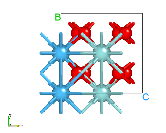
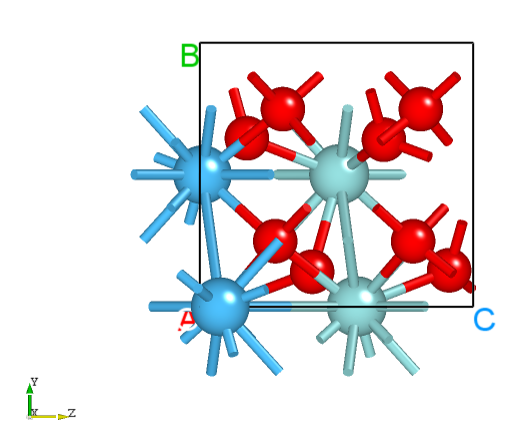
备注
When
neb.freedom = all, the options forneb.methodare QM2 or FIRE.The generation of intermediate structures can be done by calling the
neb_interpolate_structures.pyscript, as described in the “Auxiliary Tools Tutorial - Transition State Section”. After interpolation, theneb_visualize.pyscript can be called to preview the interpolated structures, and thecalc_dist.pyscript can be used to check if the distances between images are reasonable.
Run the program.
Once the input files are prepared, upload the ssneb.in and the folders containing structureNo.as files to the server and run the DS-PAW ssneb.in command as described in the structure relaxation section.
Analysis of the calculation results
After the calculation is completed based on the input files described above:
The folders containing the initial and final state structures will generate the self-consistent calculation output files such as DS-PAW.log, latestStructure00.as, and scf.h5;
The folders
Nocontaining the intermediate structures structureNo.as (folders containing intermediate structures involved in the transition state calculation, the number of intermediate structures is determined by theneb.imagesparameter) will generate output files such as nebNo.h5 and latestStructureNo.as from the structure optimization.The outermost directory will generate the files DS-PAW.log and neb.h5. The file neb.h5 is a summary of the information in the nebNo.h5 files located in the
Nofolders.DS-PAW.log : Log file generated after DS-PAW transition state calculation.
neb.h5 : The h5 data file after the transition state calculation is completed; the reaction coordinate, energy changes, and other data are saved in neb.h5. For details on the data structure, see the Output File Format Specification section.
The results of the NEB calculation can be analyzed using the python script neb.py. The analysis script should be executed within the complete NEB calculation directory. See the Auxiliary Tool User Guide section for specific instructions. The resulting reaction barrier curve should look like this:
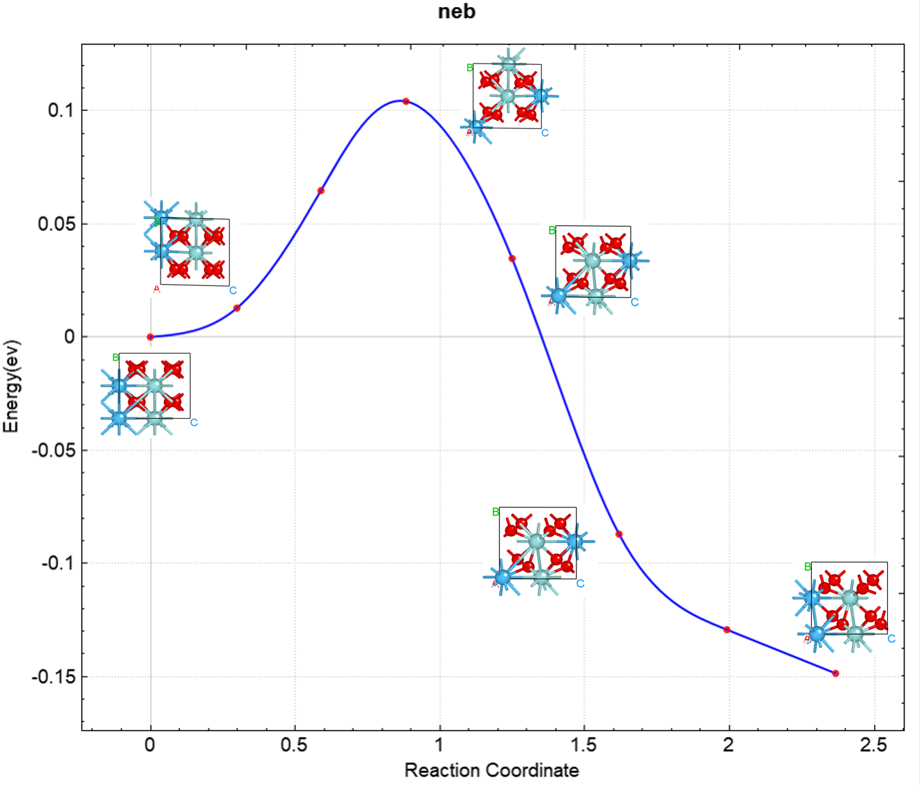
2.28 Solvation Energy Calculation
This section will use the \(H_{2}O\) system as an example to demonstrate how to calculate solvation energy under the implicit solvent model in DS-PAW.
\(H_{2}O\) solvation energy calculation input file
The input file includes the parameter file scf.in and the structure file structure.as, with scf.in as follows:
 1# task type
 2task = scf
 3#system related
 4sys.structure = structure.as
 5sys.symmetry = true
 6sys.functional = PBE
 7sys.spin = none
 8
 9#scf related
10cal.methods = 1
11cal.smearing = 3
12cal.sigma = 0.2
13cal.ksamping = G
14cal.kpoints = [1, 1, 1]
15cal.supGrid = true
16cal.cutoff = 800
17scf.convergence = 1.0e-6
18
19#implicit solvation model
20sys.sol = true
21sys.solEpsilon = 80
22sys.solTAU = 5.25E-4
23
24#outputs
25io.charge = false
26io.wave = false
27io.boundCharge = true
scf.in input parameters:
sys.sol: Controls the switch for introducing the implicit solvation model. If true, solvation effects are considered.sys.solEpsilon: Sets the magnitude of the solvent dielectric constant, set to 80 in this example;sys.solTAU: Specifies the magnitude of the effective interfacial tension per unit area, in units of eV/Å^2, with a default value of 5.25E-4. It is recommended to set this parameter to a value less than 1e-3.io.boundCharge: Switch for controlling the output of solvent-bound charge density files.
Structure file: referenced as structure.as as follows
 1Total number of atoms
 23
 3Lattice
 410.00000000 0.00000000 0.00000000
 50.00000000 10.00000000 0.00000000
 60.00000000 0.00000000 10.00000000
 7Cartesian
 8H 5.63934499 4.89541998 4.58224001
 9H 4.36065501 5.11499002 5.45934003
10O 4.65002501 4.88500998 4.54065997
run program execution
Once the input files are prepared, upload the :guilabel:`scf.in and :guilabel:`structure.as files to the server and run them, executing :guilabel:`DS-PAW scf.in according to the method described in Structure Relaxation.
Analysis of the calculation results
Based on the input files, the calculation will generate output files including DS-PAW.log, scf.h5, and rhoBound.h5.
DS-PAW.log : The log file generated after the DS-PAW implicit solvation model calculation.
scf.h5 : The self-consistent field (SCF) calculation output file in h5 format;
rhoBound.h5 : The solvent-bound charge density file obtained from implicit solvent calculations.
This example calculates the total energy \(E_{sol}\) including the solvation energy, which is calculated as follows:
Solvation Energy=E(sys.sol=true)-E(sys.sol=false)
Based on this formula, a separate calculation with sys.sol = false is required to obtain the total energy without solvation, \(E_{nosol}\). Substituting \(E_{nosol}\) into the above formula yields a solvation energy of -0.313 eV for water, which is consistent with the literature value reported in [3].
When performing calculations with the implicit solvation model, the solvent-bound charge density distribution file around the solute, rhoBound.h5, can also be obtained. This file can be post-processed using the python script trans_rho.py. For specific operations, refer to the Auxiliary Tool User Guide section. The converted visualization file can be opened in VESTA, resulting in the following isodensity surface distribution map:
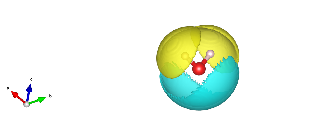
As can be seen from the figure, the distribution of solvated positive and negative shielded charge densities is located around the water molecules, forming a solvation shell, which is consistent with the model’s expectations and similar to the distribution of solvent-bound charge densities calculated by other software.
2.29 fixedpotential fixed potential calculation
This section will demonstrate how to perform fixed potential calculations in DS-PAW, using the \(Cu-slab\) system as an example.
\(Cu-slab\) Fixed Potential Calculation Input File
The input files include the parameter file fixedP.in and the structure file structure.as. The content of fixedP.in is as follows:
 1# task type
 2task = scf
 3
 4sys.functional = PBE
 5sys.structure = structure.as
 6
 7cal.ksamping = G
 8cal.cutoff = 650
 9cal.sigma = 0.2
10cal.smearing = 3
11cal.kpoints = [7,7,1]
12
13scf.convergence = 1.0e-6
14scf.max = 200
15
16sys.sol = true
17sys.solEpsilon = 78.4
18sys.solLambdaD = 3.04
19sys.solTAU = 0
20
21# Potential fixed
22sys.fixedP = true
23sys.fixedPPotential = 2.155
24
25io.charge = true
26io.wave = false
Introduction to input parameters for fixedP.in:
task: Sets the calculation type; in this example, a fixed potential calculation is performed when task=scf.sys.sol: Enables the solvation model. Fixed potential calculations need to be performed based on the implicit solvation model.sys.solEpsilon: Sets the solvent dielectric constant, which is set to 78.4 in this example.sys.solLambdaD: Uses the Poisson-Boltzmann equation and sets the Debye length. If not set, the Poisson equation is used, which does not account for the contribution of interfacial ions to the electrostatic potential.sys.solTAU: Specifies the effective interfacial tension per unit area, in units of eV/Å^2. The default value is 5.25E-4, and it is recommended to set this parameter to a value less than 1e-3.sys.fixedP: Enables the fixed potential calculation;sys.fixedPPotential: Sets the potential value for the fixed potential calculation, defaulting to the Standard Hydrogen Electrode (SHE) as the reference electrode potential. To use the Potential of Zero Charge (PZC) as the reference electrode, set the parametersys.fixedPType = PZC;
备注
Regarding the Debye length
sys.solLambdaD, its expression is \(\lambda_D = \sqrt\frac{\varepsilon \varepsilon_ok_B T}{2 c^0 z^2 q^2}\)
The Debye length for a 1M aqueous solution of +/-1 charged ions is: 3.04 Å
The structure.as file is referenced as follows:
 1Total number of atoms
 28
 3Lattice
 43.63404989 0.00000000 0.00000000
 50.00000000 3.63404989 0.00000000
 60.00000000 0.00000000 23.62132454
 7Cartesian
 8Cu 0.00000000 0.00000000 1.81702310
 9Cu 1.81702495 0.00000000 3.63404620
10Cu 1.81702495 1.81702495 1.81702310
11Cu 0.00000000 1.81702495 3.63404620
12Cu 0.00000000 0.00000000 5.46390548
13Cu 1.81702495 0.00000000 7.22885308
14Cu 1.81702495 1.81702495 5.46390548
15Cu 0.00000000 1.81702495 7.22885308
Run the program.
After preparing the input files, upload the :guilabel:`fixedP.in` and :guilabel:`structure.as` files to the server and run them, executing :guilabel:`DS-PAW fixedP.in` as described in Structure Relaxation.
Analysis of calculation results
Based on the input files described above, the calculation will generate output files such as DS-PAW.log and scf.h5.
DS-PAW.log : The log file generated after the DS-PAW calculation with a fixed potential is completed.
scf.h5 : The h5 output file corresponding to DS-PAW when task equals scf; for the specific data structure, please refer to section Output File Format Specification.
DS-PAW employs the steepest descent method for fixed-potential calculations, iteratively calculating the charge of the system for self-consistent field (SCF) calculations. The convergence process of multiple SCF calculations is written to the DS-PAW.log file. In this example, the convergence criterion is met at LOOP 5. The potential values of the system at the end of LOOP 5 are shown below:
1## FINISHED FIXEDPOTENTIAL LOOP 5 ##
2Electron                      : 149.993000
3ElectrodePotential_SHE        : 2.157747 V
4ElectrodePotential_PZC        : 2.484286 V
5ElectrodePotential_SHE(PZC)   : -0.326539 V
6Chemical Potential(electron)  : -6.757747 eV
7Grand Total Energy(sigma->0)  : -43088.518081 eV
Where
The calculated potential of the system at the end of the calculation is 2.157 V, which is close to the target potential of 2.155 V.
备注
Fixed potential calculations must be performed under the implicit solvent model; that is, when sys.fixedP = true, sys.sol must also be set to true.
Currently, fixed potential calculations are only supported when task = scf.
ElectrodePotential_SHE=ElectrodePotential_PZC+ElectrodePotential_SHE(PZC)
2.30 Wannier interpolation band structure calculation
This section will use the \(Si\) system as an example to illustrate how to perform interpolated band structure calculations using Wannier functions in DS-PAW.
Si Interpolation Band Structure Input File
The input files include the parameter file wannier.in and the structure file structure.as. wannier.in is shown below:
 1# task type
 2task = wannier
 3sys.structure = structure.as
 4sys.symmetry = false
 5sys.functional = PBE
 6sys.spin = none
 7cal.methods = 1
 8cal.smearing = 1
 9cal.ksamping = G
10cal.kpoints = [16,16,16]
11cal.totalBands = 12
12
13#wannier related
14wannier.functions = 12
15wannier.wannMaxIter = 20000
16wannier.outStep = 50
17
18#interpolated band related
19wannier.interpolatedBand = true
20wannier.kpointsLabel= [G,X,W,K,G,L]
21wannier.kpointsCoord= [0, 0, 0, 0.5, 0, 0.5, 0.5, 0.25, 0.75, 0.375, 0.375, 0.75, 0, 0, 0, 0.5, 0.5, 0.5]
22wannier.kpointsNumber = [100]
23
24io.charge = true
25io.wave = true
wannier.in Input Parameters:
task = wannier: Sets the calculation type; the new optional value wannier enables Wannier function calculations.wannier.functions: Sets the number of Wannier functions;wannier.wannMaxIter: Sets the total number of iterations in the process of solving for the maximally localized Wannier functions;wannier.outStep: Sets the step for outputting iterative results in the output file when task=wannier;wannier.interpolatedBand: Controls the switch for interpolated band calculation;wannier.kpointsLabel: Sets the high-symmetry point labels for Wannier function interpolation band fitting.wannier.kpointsCoord: Sets the high-symmetry point coordinates for Wannier function interpolation band fitting.wannier.kpointsNumber: Sets the number of k-points between high-symmetry k-points for interpolated band calculation; for example, setting the parameter towannier.kpointsNumber = [100], the number of k-points between the high-symmetry points G and X is 100, which is used to determine the k-point density; the code performs equally-spaced k-point sampling between high-symmetry points X and W, W and K, K and G, and G and L. The actual number of k-points can be found in the parameter printing section of DS-PAW.log.
The structure.as file is referenced as follows:
1Total number of atoms
22
3Lattice
40.00 2.75 2.75
52.75 0.00 2.75
62.75 2.75 0.00
7Direct
8Si -0.125000000 -0.125000000 -0.125000000
9Si 0.125000000 0.125000000 0.125000000
备注
The initial projection is set in the structure.as file. First, add the WannProj tag on line 7, and then write the initial projection orbital names after the atomic coordinates. Refer to the Wannier section in Parameters Explanation for the recognizable projection orbital names for DS-PAW.
In this example, initial projections are not customized, and the program randomly selects them. If you need to define initial projections, you can refer to the following format.
The structure.as file for custom initial projection orbitals is referenced as follows:
1Total number of atoms
22
3Lattice
40.00 2.75 2.75
52.75 0.00 2.75
62.75 2.75 0.00
7Direct WannProj
8Si -0.125000000 -0.125000000 -0.125000000  [s,p,sp3-1,sp3-2]
9Si 0.125000000 0.125000000 0.125000000     [s,p,sp3-3,sp3-4]
备注
When customizing initial projection orbitals, the total number of projection orbitals in the structure.as file must equal the number of Wannier functions (wannier.functions), otherwise the program will report an error.
In this example, the total number of projected orbitals is 2*(1+3+1+1) = 12, which is consistent with the wannier.functions = 12 parameter setting.
For atoms without the need to set initial projection orbitals, simply write `[]` after the corresponding coordinates.
In this example, cal.totalBands is set to 12, so 12 cores are required when submitting the calculation.
run the program
Once the input files are ready, upload the wannier.in and structure.as files to the server and run the DS-PAW wannier.in following the method described in structure relaxation.
Analysis Results Analysis
Based on the input files described above, the calculation will generate output files such as DS-PAW.log and wannier.h5.
DS-PAW.log : The log file generated after DS-PAW completes the Wannier interpolation band calculation.
wannier.h5 : The h5 output file corresponding to the Wannier function interpolated band structure calculation; for details on the data structure, see the Output File Format Specification section;
You can use the Auxiliary Tool User Guide –> band data processing –> bandplot.py script to directly plot the Wannier interpolated bands, reading the wannier.h5 file.
You can also use bandcompare.py to compare the Wannier interpolated band structure with the DFT band structure. See Auxiliary Tool User Guide for specific operations. The band comparison effect should be as follows:
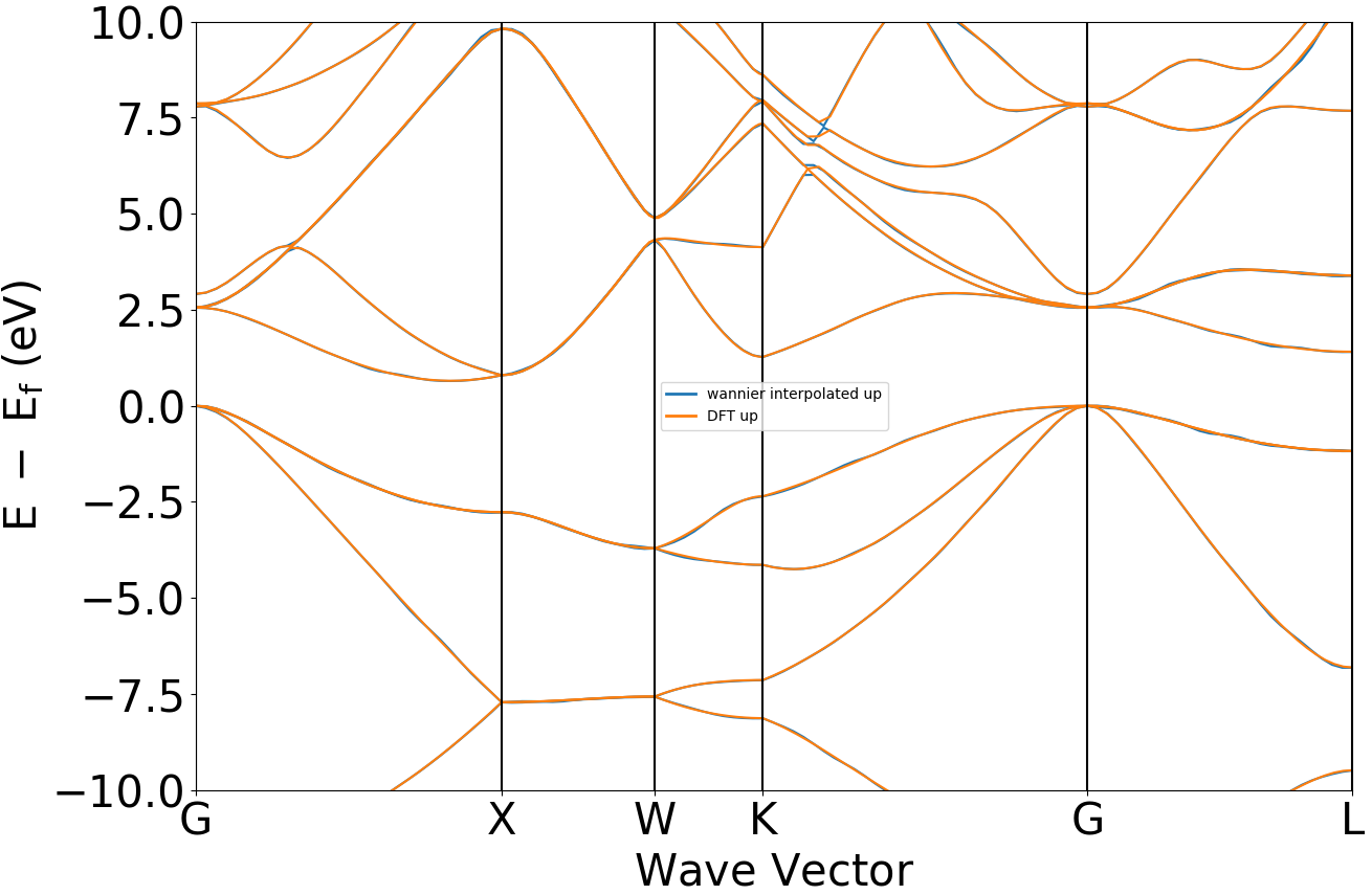
备注
Wannier calculations do not support opening pob, and the number of DFT bands calculated (cal.totalBands) changes with the number of cores (cores) used. Therefore, it is recommended that the number of cores used for Wannier calculations be consistent with the cal.totalBands parameter.
When the number of Wannier functions (wannier.functions) is less than cal.totalBands, the disentanglement process is required during the maximal localization of Wannier functions. In this case, if the user does not define an energy frozen window (wannier.disFrozWin), the program will perform the calculation using the default frozen window.
If a custom Frozen Window is defined, the number of bands included in `wannier.FrozWin` cannot exceed the number of `wannier.functions`; otherwise, the program will report error E4024. At the same time, the rationality of the window needs to be ensured, or good fitting results cannot be obtained.
The 2023A version of DS-PAW does not support Wannier calculations with the spin type set to non-collinear.